
The year is 1888, and the infamous serial killer Jack the Ripper is haunting the streets of Whitechapel. As a detective in Victorian London, your mission is to track down this notorious criminal – but you have a problem. The only information that you have to go on is the map below, which shows the locations of crimes attributed to Jack. Based on this information alone, where on earth should you start looking?

The fact that Jack the Ripper was never caught suggests that the real Victorian detectives didn’t know the answer to this question any more than you do, and modern detectives are faced with the same problem when they are trying to track down serial offenders. Fortunately for us, there is a fascinating way in which we can apply maths to help us to catch these criminals – a technique known as geospatial profiling.
Geospatial profiling is the use of statistics to find patterns in the geographical locations of certain events. If we know the locations of the crimes committed by a serial offender, we can use geospatial profiling to work out their likely base location, or anchor point. This may be their home, place of work, or any other location of importance to them – meaning it’s a good place to start looking for clues!
Perhaps the simplest approach is to find the centre of minimum distance to the crime locations. That is, find the place which gives the overall shortest distance for the criminal to travel to commit their crimes. However, there are a couple of problems with this approach. Firstly, it doesn’t tend to consider criminal psychology and other important factors. For example, it might not be very sensible to assume that a criminal will commit crimes as close to home as they can! In fact, it is often the case that an offender will only commit crimes outside of a buffer zone around their base location. Secondly, this technique will provide us with a single point location, which is highly unlikely to exactly match the true anchor point. We would prefer to end up with a distribution of possible locations which we can use to identify the areas that have the highest probability of containing the anchor point, and are therefore the best places to search.
With this in mind, let’s call the anchor point of the criminal z. Our aim is then to find a probability distribution for z, which takes into account the locations of the crime scenes, so that we can work out where our criminal is most likely to be. In order to do this, we will need two things.
- A prior distribution for z. This is just a function which defines our best guess at what z might be, before we have used any of our information about the crime locations. The prior distribution is usually based off data from previous offenders whose location was successfully determined, but it’s usually not hugely important if we’re a bit wrong – this just gives us a place to start.
- A probability density function (PDF) for the locations of the crime sites. This is a function which describes how the criminal chooses the crime site, and therefore how the criminal is influenced by z. If we have a number of crimes committed at known locations, then the PDF describes the probability that a criminal with anchor point z commits crimes at these locations. Working out what we should choose for this is a little trickier…
We’ll see why we need these in a minute, but first, how do we choose our PDF? The answer is that it depends on the type of criminal, because different criminals behave in different ways. There are two main categories of offenders – resident offenders and non-resident offenders.
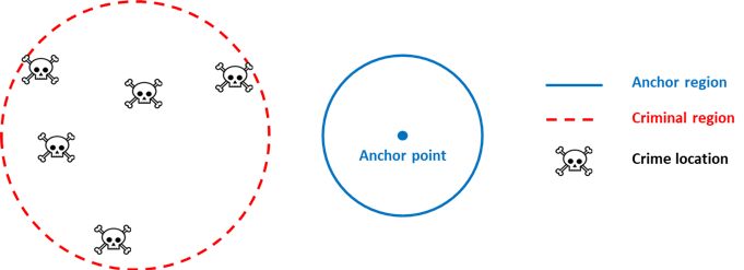
Resident offenders are those who commit crimes near to their anchor point, so their criminal region (the zone in which they commit crimes) and anchor region (a zone around their anchor point where they are often likely to be) largely overlap, as shown in the diagram:

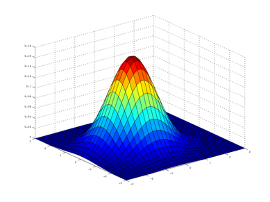
If we think that we may have this type of criminal, then we can use the famous normal distribution for our density function. Because we’re working in two dimensions, it looks like a little hill, with the peak at the anchor point:
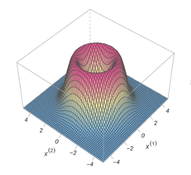
Alternatively, if we think the criminal has a buffer zone, meaning that they only commit crimes at least a certain distance from home, then we can adjust our distribution slightly to reflect this. In this case, we use something that looks like a hollowed-out hill, where the most likely region is in a ring around the centre as shown below:
The second type of offenders are non-resident offenders. They commit crimes relatively far from their anchor point, so that their criminal region and anchor region do not overlap, as shown in the diagram:
If we think that we have this type of criminal, then for our PDF we can pick something that looks a little like the normal distribution used above, but shifted away from the centre:

Now, the million-dollar question is which model should we pick? Determining between resident and non-resident offenders in advance is often difficult. Some information can be made deduced from the geography of the region, but often assumptions are made based on the crime itself – for example more complex/clever crimes have a higher likelihood of being committed by non-residents.
Once we’ve decided on our type of offender, selected the prior distribution (1) and the PDF (2), how do we actually use the model to help us to find our criminal? This is where the mathematical magic happens in the form of Bayesian statistics (named after statistician and philosopher Thomas Bayes).
Bayes’ theorem tells us that if we multiply together our prior distribution and our PDF, then we’ll end up with a new probability distribution for the anchor point z, which now takes into account the locations of the crime scenes! We call this the posterior distribution, and it tells us the most likely locations for the criminal’s anchor point given the locations of the crime scenes, and therefore the best places to begin our search.
This fascinating technique is actually used today by police detectives when trying to locate serial offenders. They implement the same steps described above using an extremely sophisticated computer algorithm called Rigel, which has a very high accuracy of correctly locating criminals.
So, what about Jack?
If we apply this geospatial profiling technique to the locations of the crimes attributed to Jack the Ripper, then we can predict that it is most likely that his base location was in a road called Flower and Deane Street. This is marked on the map below, along with the five crime locations used to work it out.

Unfortunately, we’re a little too late to know whether this prediction is accurate, because Flower and Deane street no longer exists, so any evidence is certainly long gone! However, if the detectives in Victorian London had known about geospatial profiling and the mathematics behind catching criminals, then it’s possible that the most infamous serial killer in British history might never have become quite so famous…
Francesca Lovell-Read

[…] by /u/tomrocksmaths [link] […]
LikeLike
[…] Find out how this method can be used to pinpoint the probable home of ‘Jack the Ripper’ courtesy of Tom Rocks Maths intern and Oxford University student Francesca Lovell-Read here. […]
LikeLike