If you’ve ever had a sprinkler in your garden and like me used to run through it in the summer as a kid, you’ll have noticed the different pattern of the water for when the sprinkler is on compared to when it’s off (or maybe I was just a weird kid). When not rotating, the water shoots out in a straight line in all directions. If you stand at the centre and look directly North, the water will shoot out in a straight line and land directly North of where it started. Now if you turn the sprinkler on so that it starts rotating the patterns become curved. As the sprinkler turns it will still release water directly North, but because of the rotation a sideways force will push it to the left as it’s released (for a sprinkler going anticlockwise). This gives a curved path and the water will actually land a fair bit to the left (or East) of direct North.

The same thing that happens with your sprinkler is also happening with the Earth. This sideways force is quite weak so it only really affects large distances, which means Usain Bolt running the 100 m is safe from its effects, but Mo Farah running the 10,000 m – he will feel it. And the force, called the Coriolis force, is stronger the further you go North or South from the equator. That means it’s very important in controlling how river water moves once it enters into the ocean. As I hinted at in the previous article, it is one of the most important parameters affecting the motion of the water and as such we have to make sure that it is represented correctly in the lab experiments.

For my experiments we did this by mounting a giant fish tank (literally the best way to describe it) on top of a turntable whose speed could be controlled by a computer. The Earth rotates at a very high speed of 1000 mph, but the actual Coriolis force arising from the rotation is relatively small at f = 0.0001 s^-1 at mid-latitudes (i.e. around the UK). As with building a scale model of a river in the lab, we can’t just scale down the Coriolis force. We know that it’s important because without it the water moves in a completely different direction and so we have to make sure it’s represented in the experiments, but knowing what value to use requires a little more thought.

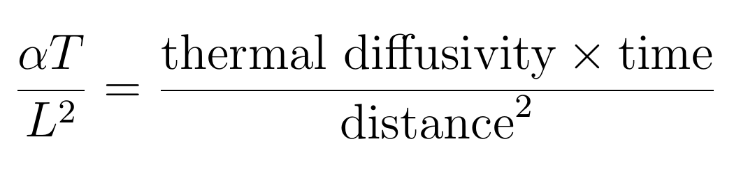
This is where we come to the real heart of applied maths – scaling analysis – and it works as follows… Suppose we have 3 parameters that we know are important in our problem, i.e. without any of them the outcome changes dramatically (think of a sprinkler with no rotation for example). Taking one of my favourite problems of the spread of heat through a rod, we might expect that the material the rod is made from and the length of the rod will both affect the time it takes for the heat to spread out. In fact, the particular property of the material that we want here is the thermal diffusivity – a fancy way of saying how quickly the material heats up. Now, if we look at the units of these three quantities, we have time T in seconds (s), length L of rod in metres (m) and thermal diffusivity α in metres squared per second (m²s^-1). Fiddling around with these quantities we can create a dimensionless parameter (one without units) given by

and this then tells you that the time taken relates to the length and the thermal diffusivity in the following way

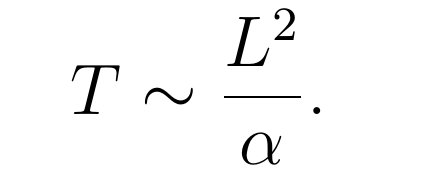
At this point it may seem quite random and not really of any use, but when you actually write out the full problem mathematically and solve the resulting system of equations, your solution is given by

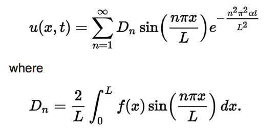
The only part we need to look at is the exponential term (e) as this is the only part of the solution that has a dependence on time (t). You’ll notice that the exponential power is the same as our dimensionless quantity above (plus some numbers n and π). Solving the equations is great if you need a full solution, but if you only need certain information, like which factors affect the time taken, then we actually already had that from our scaling analysis T ∼ L²/α. To speed up the spread of the heat and decrease the time (T) we just increase the thermal diffusivity (α) or we decrease the length of the material (L). The solution tells us this, but so too did our scaling analysis (with much less effort).

Hopefully you’ve spotted that the trick is to first identify the parameters that are most important to a given problem, and then to combine them in such a way that all of the units disappear – making them dimensionless. For a river our parameters might be rotation f in s^-1, the volume flux Q (amount of water flowing out of the river) in m³s^-1 and the density difference between the freshwater of the river and the saltwater of the sea, which we represent as the reduced gravity g’ with units ms^-2. Combining the units, we find that the dimensionless parameter is given by

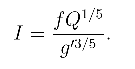
For real rivers we can compute the value of I, and when designing the lab experiments we need to make sure that the value of I for the experiments matches up with the values for the real rivers – that’s the key to capturing the most important real-world behaviour. It also has the advantage of allowing us to vary the parameters by quite a large amount depending on what is easiest to achieve in the lab. For example, a volume flux of 2,200,000 cm³s^-1 of the River Rhine cannot be used in the lab (the maximum I used was about 100 cm³s^-1), but what we can do is increase or decrease the other parameters to keep the value of I about the same. Here we can increase f and increase g’ which are must easier to do in the lab, we just need a fast turntable and some seriously salty water, which brings me nicely onto our next topic: my experimental setup.

All of the articles explaining my PhD thesis can be found here.