
Charlie Ahrendts (Image: Mathworks)
Let us continue our journey to meet a new civilization… We find them on a gas giant, similar to Jupiter. The first thing that grabs our attention is the omnipresence of movement. Looking at the ground we see that it is in a constant slowly flowing motion, and it doesn’t seem to bother the local inhabitants. So, what can we learn from them and how would their mathematics differ from ours? We could assume that they would have adapted not only themselves, but also their maths to their environment. Describing and understanding flow would have a much higher importance than things like geometry.
For us humans, describing and understanding flow poses one of the hardest mathematical problems we have ever come upon. There is a very famous set of equations, called the Navier-Stokes equations that describe the motion of liquids and gases. Although we have known about them for over 150 years, we are only able to solve them for a few, very specific cases. Understanding the aliens’ approach to this problem and its solutions could help us to gain a deeper understanding about our own world. And maybe their greatest problem lies in the lengths of the sides of a triangle. Who knows what we might learn from each other…
Partial Differential Equations
Partial differential equations pose some of the hardest problems to solve in mathematics, but what exactly are they? And what makes them so difficult? Let us explore these questions with the example of the heat equation.
A partial differential equation, or PDE in short, is an equation that depends on the derivatives of some of its variables. This means that it looks at the rates of change of certain properties, instead of the whole system. Let us imagine a one dimensional or very thin metal rod. This rod is heated in some places and cooled down in others. We want to find an equation that describes how the heat distribution will evolve – this is called the ‘Heat Equation’.
We know that the temperature of the rod depends on two factors: time and position. Because our idealised rod is one dimensional, we only need one variable to describe any point on the rod. Let us call this variable x. Of course we can’t have one dimensional objects in the real world, but it often is helpful to start with a simpler case and then expand it to higher dimensions. The second important factor is time. If we leave the rod for some time, some regions will have cooled down and others will have heated up. Since it describes the evolution over time, we will name this variable t.
Another way to understand these two variables is the following: Whenever I fix t on some value, let’s say 5 seconds, varying x will allow me to see the temperature of every point on the rod after 5 seconds. If, on the other hand, I fix x on some value, say x = 1 cm, changing t will allow me to see how the temperature changes with time at the point exactly 1 cm along the rod. The function that describes the temperature at any time and any position along the rod will be denoted by T(x,t) with T being temperature, x being position and t being time. Keeping this in mind, we can finally look at the actual equation:

One of the things you may notice is that this does not look like most equations we know. Perhaps you were expecting something that looks more like T(x,y) = something – and we are indeed working towards that, but for now we are stuck with this, so let’s try to make some sense out of it.
If you have studied maths at A-level you might remember learning about derivatives. Taking a derivative equates to finding the rate of change of some function with respect to a certain variable. Imagine drawing a graph of a moving car. On the x axis we have time and on the y axis the distance from the starting point. Taking the derivative means describing the change of position over time, or in other words, the velocity. In the example graph shown below the distance changes at a constant rate over time and so the gradient, or derivative, is simply a constant.

The first part of the heat equation does the same thing – it describes the rate of change of temperature with respect to time. We could also write it as ΔT / Δt which is read as ‘delta T over delta t’. In essence we are asking how a tiny step forwards in time changes the temperature at a fixed point. If we look at the hottest point on the rod and compare its temperature at lets say 5 seconds and a very short time later, the rod will have cooled down a tiny bit at that point. The smaller the change to the input (time in this case) the more accurate the output. With a few tricks (and a proper treatment of limits), we can make that tiny change approach zero and get an accurate result of the rate of change at that exact time.
On the other side of the equation, we have α Δ2T / Δ x2. α is what we call a material constant – it simply describes how fast the temperature will average out in a given material. A metal rod for example is a heat conductor, and therefore it will heat up or cool down relatively quickly. A plastic rod on the other hand would take much longer to get to the same temperature everywhere because it functions as an insulator.
You might have noticed that the second part of the term looks very similar to the first part of the equation we talked about. And you would be right in thinking so. We are again taking a derivative, only this time with respect to x. We are no longer looking at the effects of a tiny change in time, but rather a tiny increase in x, or in other words a small step right on the rod. The other difference is that we have an added square. This means that we take the second derivative, the derivative of the derivative. Since that is not at all intuitive, there is another way to think of it in this context.
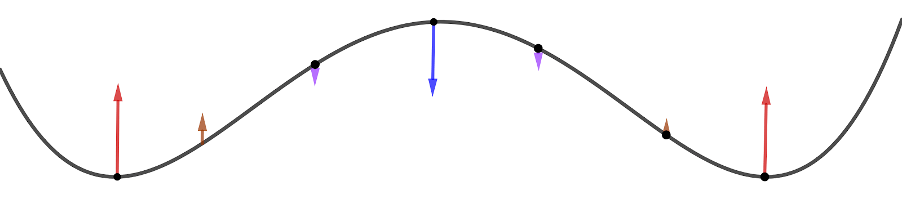
Imagine picking one point on the rod and measuring its temperature. We call that temperature T1. We now measure the heat directly left of T1 and directly right of it and call those points T2, and T3 . Now that we have three points that are very close together, we can take the outer ones and average their temperatures. If we compare this value with T1 there are three possibilities of what can happen. If T1 is smaller than the average of T2 and T3 it means that it is colder than its surroundings, so it will heat up. If it is hotter than the average temperature around it, it will cool down, and if it is the same, there is no need for it to change, so it will stay constant. Taking the second derivative in this context is in essence the same as looking how much hotter or colder any point on the rod is, compared to its neighbours and how it changes accordingly.

If we now take the whole equation into consideration, we can see that it describes how the change of temperature depends both on the change in time and position. Keep in mind that we are still talking only about change. If we look at the equation, we can see that a big change in temperature over a small amount of time, or in other words a large value on the left, means that there has to be a big number on the right as well and we can illustrate this connection really nicely as follows.
Let us suppose we have two identical rods. One where one end is heated to 50° and the other where one end is heated to 100°. The other end will have the same temperature in both cases. If we move along the rod at t=0, the temperature will change much more in the hotter rod, just because the difference between the hottest and coldest point on the rod is greater than that of the other one. If we now look at a single point on the rod and how it changes over time, we will again see that the change is greater in the rod whose end was heated up to 100°. And this makes a lot of sense, since we have more energy in the system which can heat up or cool down the rod.
Now that we have hopefully understood the equation, I want to briefly talk about what a solution might look like. Note that we have so far only talked about changes in the temperature T. Finding a solution means finding some function T(x,t) that matches the requirement of the PDE, namely that its time-derivative (rate of change with respect to time) is proportional to its second space-derivative (change with respect to the rate of change of position). Unfortunately, finding such functions is often not very easy. For example, there are PDEs like the aforementioned Navier-Stokes equations where we only have solutions for very specific conditions. This is fortunately not the case for the heat equation, where general solutions do exist, which can be found using the technique of Fourier Series. But, that is a topic for another day.
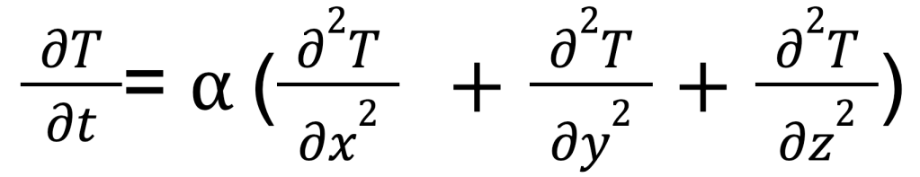
Now that we have a rough idea of what the heat equation is, and why we use PDEs to describe a change in some value that depends on multiple variables, you will see that many similar equations follow the same formula. If we want to make the model more realistic, for example by expanding our differential equation into three spatial dimensions, we just add terms for the y and z values, with the rest of the equation staying the same. With this we can describe heat flow in any three dimensional object as follows:
Although often hard, or sometimes almost impossible to solve, partial differential equations are a powerful as well as versatile tool. They allow us to describe and understand heat distribution, random motion of particles, fluid dynamics and even stock market analysis to name just a few examples – the possibilities are endless!

[…] Stop 2: Fluid Planet […]
LikeLike