James Robinson – 2022 Teddy Rocks Maths Essay Competition Commended Entry

Find the nearest circular object, it could be anything, the steering wheel of your car, a tin can, a roll of tape, as long as its circumference (perimeter) divided by its diameter (width) is approximately the magical, mystical pi (3.1415926535….). Now trace your finger around the outer edge of this circular object, paying close attention to the height of your finger as you complete one revolution. For those playing along at home, I challenge you to try and draw a graph of your finger’s journey. On the y-axis plot the height of your finger and on the x-axis plot the distance you have travelled around the perimeter. There are no bonus points for accuracy but what is important is the general shape of the curve you have produced.

With or without knowing it you have just produced a sinusoid. This is a periodic, continuous curve, often called a ‘sine wave’. Most of us have come across this wave in two of its infinitely many forms: the sine and cosine functions.

These functions are routinely taught in mathematics class and that is for a reason, these graphs are all around us and whether you like it or not it is useful to understand the beauty of these curves. Understanding the fundamental nature and applications of these curves can help us understand the world around us and gain a deeper appreciation for the laws of physics and the maths that can help model them.

If you hadn’t guessed by now the link between the seemingly arbitrary collection of words in the title is the sinusoidal function.

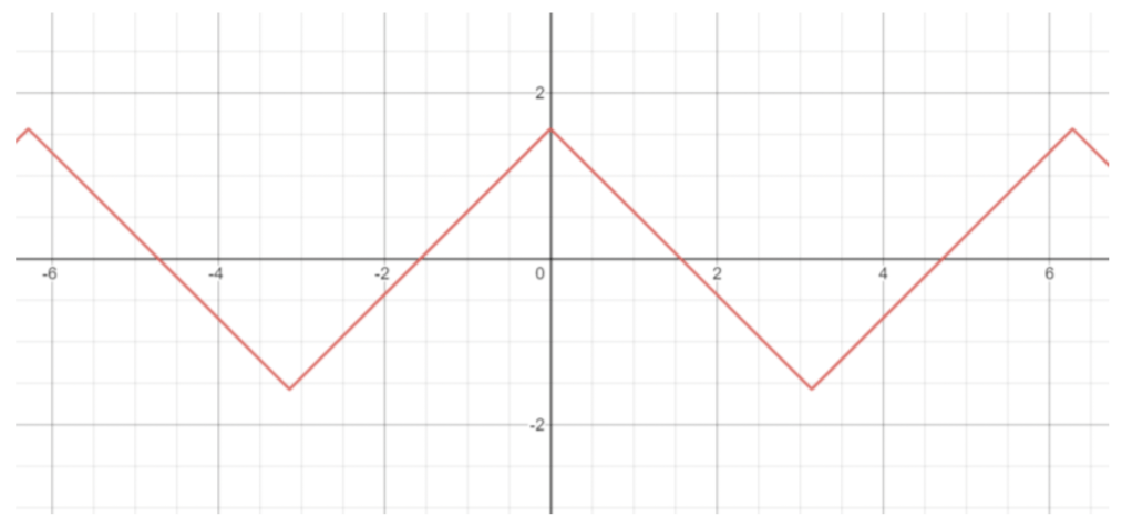
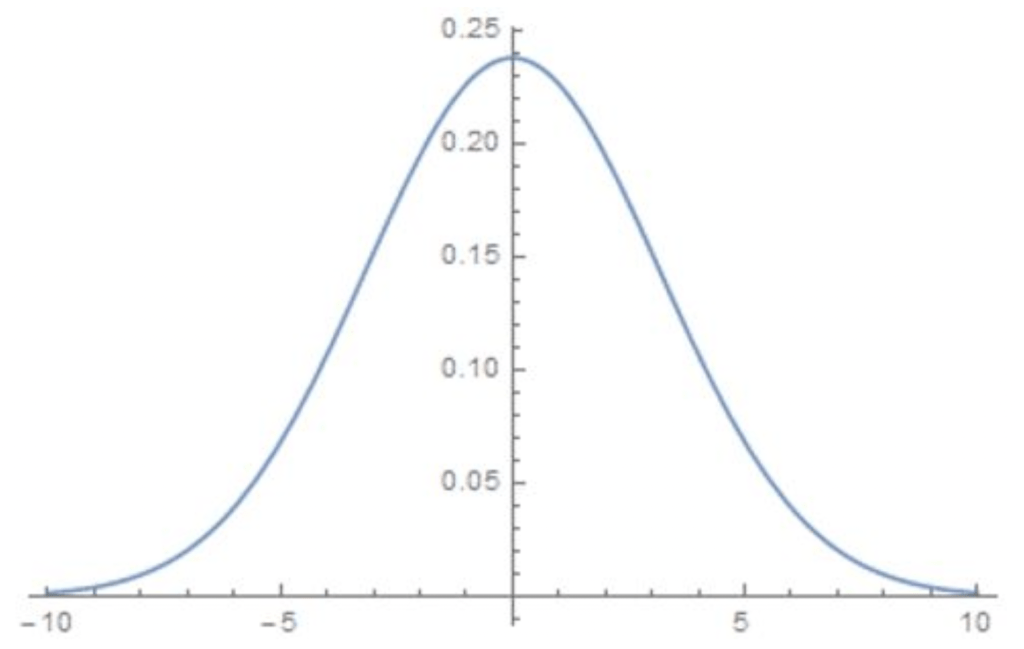
Now, the sinusoid you drew before should have looked something like this:

We can see some of the key features of the sinusoid, which in this case in a sine graph. This may seem pretty boring but I promise you once you understand what we can do with these functions it get a whole lot more exciting.

One mathematician who made great use of the sinusoidal functions is Joseph Fourier. In the early 1800s Joseph Fourier realised the limitless possibilities of adding these waves together as a way of approximating and modelling other, more complex periodic functions. He invented the Fourier series which in essence describes a way of representing a complex periodic function, like the human voice or the chime of a bell, as the sum of infinitely may sinusoids with differing amplitudes and frequencies. The equation is as follows:

To simplify, the a_n and b_n refer to a list of values that are used as coefficients for a particular frequency of sine and cosine respectively (note a value of 0 means that this particular frequency does not exist in the function g(t). Next all these values are summed up by the use of the capital sigma and then a constant (c) is added. In simple terms we are adding infinitely many sine and cosine functions together!

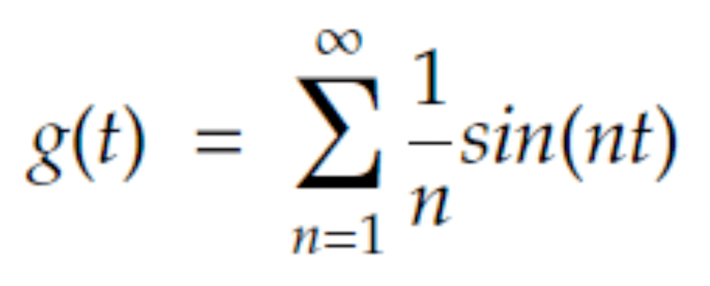
Now to show the power of this series I want to show possibly the most extreme case of this series working. Let c be any arbitrary number. Now let b_n = 0 for all values of n. For all even values of n let a_n = 0 and for all odd values of n let a_n = 1/n and f also n. This now can be expressed by a single summation as follows:

I have used the term ‘2n-1’ as a short cut to generate only odd values of n as all even terms sum to zero. Now graphing this we get:

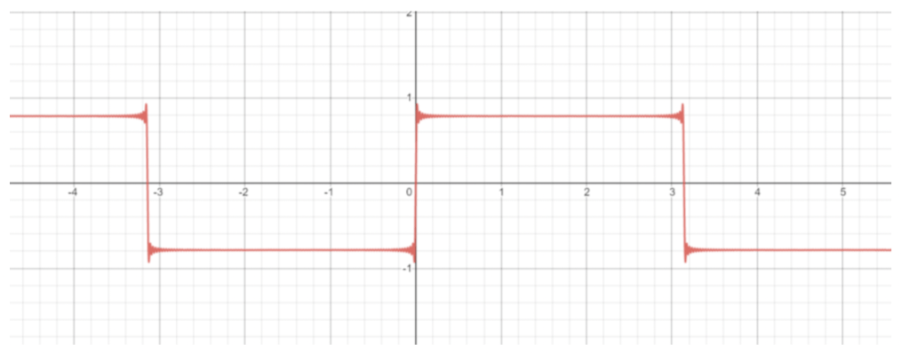
Not impressed? It has been proven this series converges to what is known as a square wave. Square waves are normally found only in the most digital applications, in your computers and electrical timers as they apply well to binary as they are either high or low. What is so outstanding about this is that we have taken something so pure as a sine wave, something so inherently physical that it can model the smallest vibrations of particles to the gravitational waves that spread out through the galaxy, and infinitely add them we can converge on something so discrete and digital.

Another place you may have seen a square wave is in a process known as subtractive synthesis. This is a method of sound design that takes a waveform and remove pieces of it to create a sound. There are 4 basic waveforms in this type of synthesis the sine wave (a pure sine function) the square wave (as shown above) and two more. To prove the power of the Fourier series these two can also be approximated by the series I will show them being produced by the series.

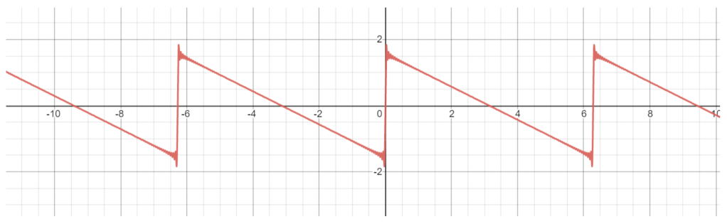
First the sawtooth or, as it is sometimes called. For all values of n:

• a_n = 1/n
• b_n = 0
• f = n

The Fourier series simplifies to:

And graphed to n = 100 we get a saw-tooth wave:

And finally the triangle wave: For odd values of n:

• a_n = 0
• b_n = 1/(n²)
• f = n

For even values of n:

• a_n, b_n = 0
• f = n

The Fourier series simplifies to:

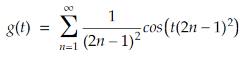
And graphed to n = 100 we get the triangle wave:

With these four waves forms being both musically useful and mathematically interesting most would assume both mathematicians and musicians would have been satisfied with the tools they were given. Most electronically synthesised music traditionally used one of more of these waves but in the late 1960s John Chowning decided he’d had enough of the boring linear coefficients used in the Fourier series and decided instead to multiply sinusoids together to make more interesting sound. This is known as frequency modulation where a carry signal modulates (changes the amplitude) of a signal, which in this case is another sinusoid. Although not a new technology, FM radios had been invented in 1933 by Edwin Armstrong, Chowning was the first to experiment with what is now known as FM synthesis.

Picture this: it’s November 1984 and A-ha have just released their smash hit ‘Take on me’. You become immersed in the groovy bass line, the glistening leads and the swelling pads. Ahh the good old days! In fact what you are hearing is the power of FM synthesis and more specifically the Yamaha DX7. This instrument essentially works by addition and multiplication of 6 individual sine waves to replicate sounds such as flutes, organs, electric pianos and even the human voice. These are all produced by 32 individual algorithms but it is possible to program your own and with a lot of maths it is possible for the range of sounds to be broadened to, as the Fourier series suggests, any periodic function.

Not happy with just creating simple periodic functions with an infinite sum of sinusoids, Joseph Fourier decided to extend his series to all functions. However, he wasn’t finished with this, instead he wanted a way of essentially extracting the frequencies that made up these functions. Simply put he wanted to be able to take a function f(t) and manipulate it in some way as to produce a function that was a representation of the f(t) as frequency and amplitude (which can be used to find the f, a_n and b_n for the Fourier series that approximates f(t)). The result of this was the Fourier transformation.

Technically, the Fourier transform is a complex valued function that can transform a space or time domain to a frequency domain or the other way, this is what is so useful about this transform. The Fourier transform has the generalised equation:

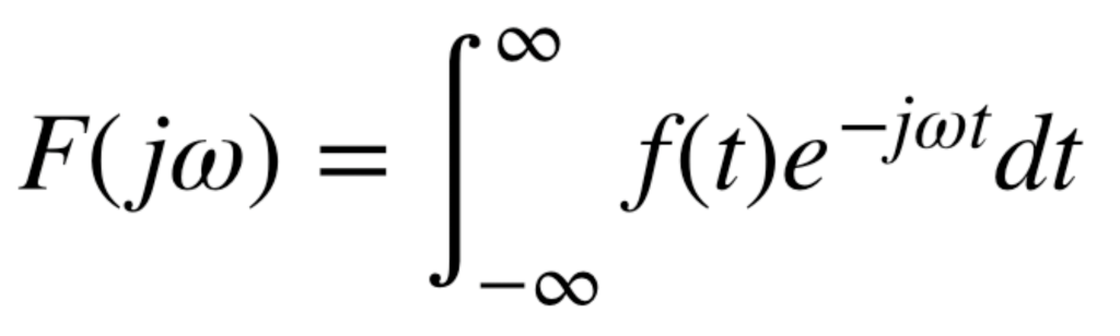
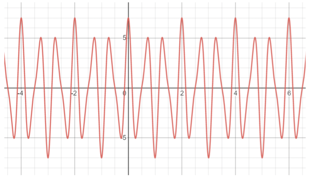
This may look extremely daunting at first and some of the maths to explain this is difficult but there is a logical way of understanding this transformation. One the most basic level we have a function and we plot it as normal. Let f(x) = 5 cos(3πx) + 2 cos(5πx). I hope from here it is easy to see that if we break f(x) down into its underlying frequencies we have one cosine function of ‘3’ and another of ‘5’ with the respective amplitudes being ‘5’ and ‘2’. With the Fourier transform we get F(x) which displays this frequency and amplitude information. The function f(x) has been plotted in red below:

The Fourier transformation of f(x), labelled F(x), has been plotted below in purple:

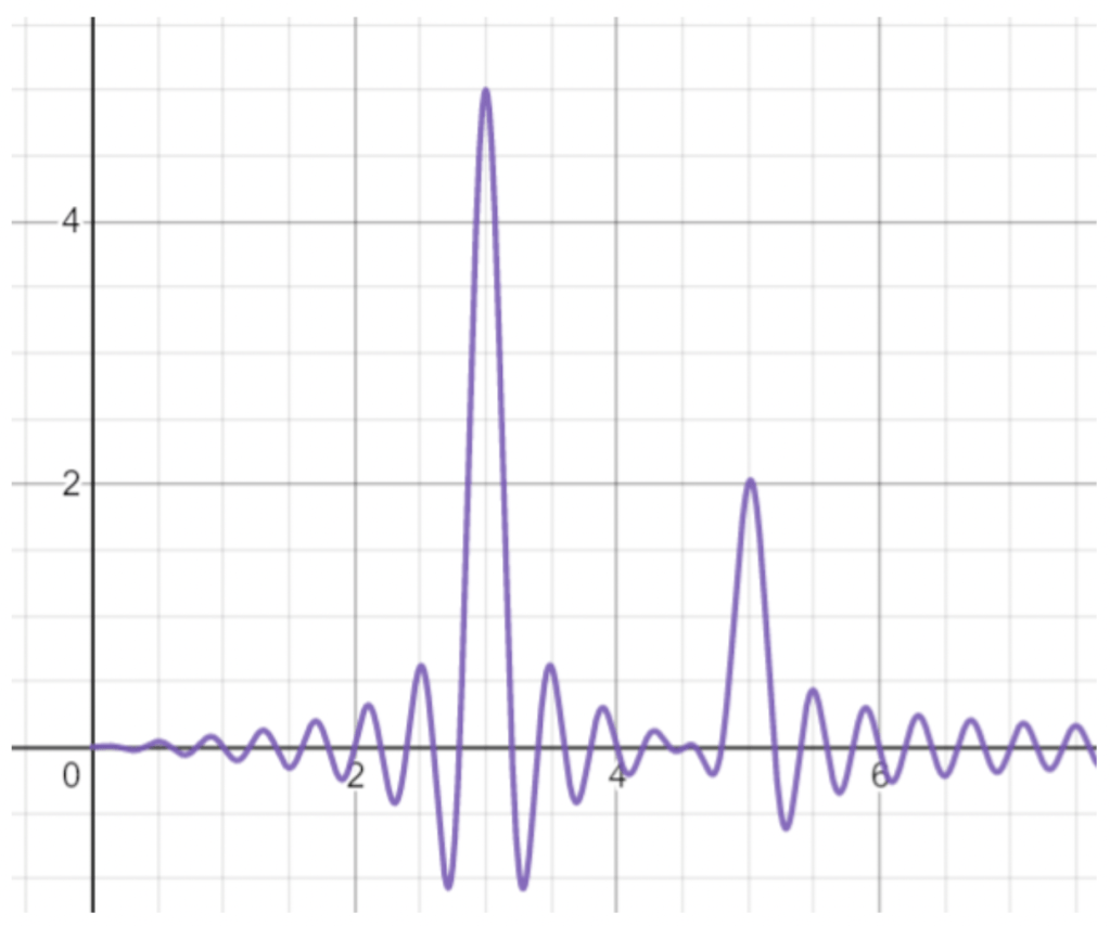
We can see that the large spikes in the transformed function have maximums at (3,5) and (5,2) which, due to the x-axis being representative of increasing frequency and y-axis being amplitude, we see that this perfectly represents our original function f(x) in terms of frequency and amplitude. Or, to be more specific, transforms f(x) from the frequency domain to the frequency and amplitude domain.

You may have expected to see two vertical lines like this:

The reason the transform doesn’t look like this is because the Fourier transform outputs a continuous function, so the graph above, which is discrete, couldn’t be outputted by a Fourier transformation (although a Fourier series could be used to approximate this!). A curious by-product of this approach means that values around the maximums on the transformation can be used to approximate the original function. However, this also introduces an uncertainty in the frequency and values around the actual frequency can be used to approximate the original function. This can be used to explain Heisenberg’s Uncertainty Principle. This is a principle that forms the backbone of quantum mechanics and simply put states that the more accurately you know a particle’s position the less accurately you know its momentum. When this idea is married with the fact that particles have wave like properties in quantum mechanics we can apply the Fourier transform to these particles. Take any particle and let its position be defined by the function p(x). Now we have a position value we need to be able to also model its momentum. How do we do this? You guessed it, we use the Fourier transformation of p(x). Think of what was once frequency to now be momentum. Say we have a particle and we are able to accurately measure it’s position, reducing the uncertainty in this measurement, we could show the position of the particle as such:

Where we can think of the width of the spike as the uncertainty in the position and in this case it is fairly low. We know we can obtain the momentum of the particle by using a Fourier transform on it and plotted it looks something like this:

If we apply the same rules that the width of the spike is the uncertainty it is obvious to see that the uncertainty in momentum is very high. We would then naturally try to decrease this uncertainty by making the momentum values have less uncertainty, by measuring the particle’s momentum more accurately, making the spike thinner. If we do this we could model momentum as such:

From here it seems as though we have solved the problem until we remember that the Fourier Transform can work in either direction so we can therefore obtain a model for the position of the particle from this which would be as follows:

The problem is that if we lower the uncertainty in one parameter, we increase the uncertainty in the other. This is the essence Heisenberg’s uncertainty principle and is what causes many quantum phenomena’s like quantum tunnelling (where particles can effortlessly pass through barriers), has been used to explain quantum fluctuations and thus Hawking Radiation. Since it’s first formulation in 1927 the uncertainty principle and the development of quantum mechanics has revolutionised the field of theoretical physics, leading to such theories as M-theory and string theory.

In summary, I hope you enjoyed this crash course in all things sinusoids and can now appreciate there use in maths, physics and the composition of timeless hits!