
Molly Roberts
At last! You’ve packed everything in the car, your ABBA CD is ready to go, you’ve checked your rear view mirror, and you go to put your destination in the sat nav. It asks whether you want the shortest route or the quickest route, and you have an existential crisis because all you want to be doing right now is lying on a sunbed drinking a diet coke whilst slathered in factor 50 suncream, and your brain is still fried from trying to use bubble sort to get your bags in the car. (See part 2 here). Perhaps it would be easier if you understood how the sat nav calculates its routes, so you don’t get annoyed later when you get stuck in traffic because you chose ‘shortest’ instead of ‘quickest’.
Surprise, surprise, it’s by using an algorithm. Put your seatbelt on and buckle up – it’s time to learn how to be cleverer than your sat nav…
Dijkstra’s Algorithm
Alright, this algorithm is probably the most complicated one I’m going to talk about in this series, and so instead of writing out a list of instructions, I think it would be much easier to show you how it works with a simple example:
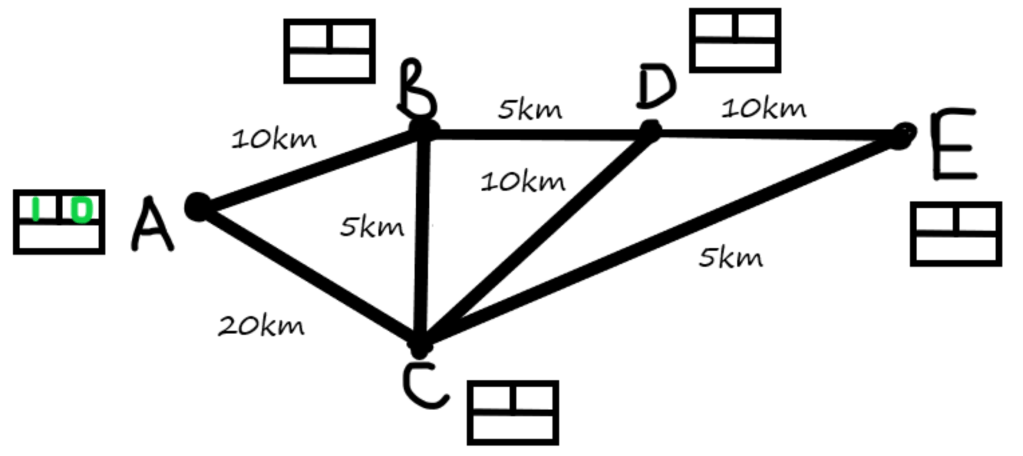
Imagine we are trying to get from town A to town E. Several places we could go through along the way are towns B, C, and D. We will use a simple version of the map as follows:
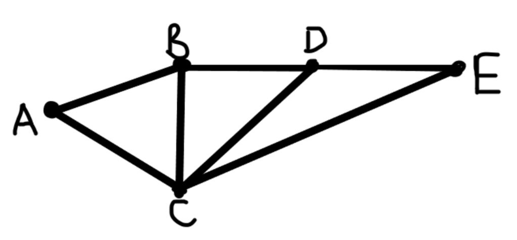
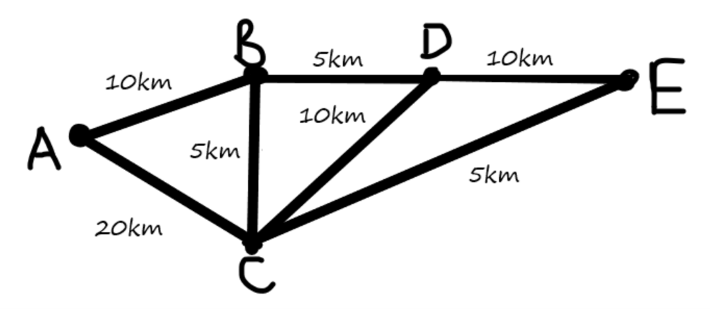
In this diagram, the dots (or nodes) mean towns, and the lines represent the roads connecting them. In this situation, we might choose to consider the distance we have to travel to get directly between each town on the map. We can put this in a table, and also add it to the diagram:
| A | B | C | D | E | |
| A | – | 10 km | 20km | No direct route. | No direct route. |
| B | 10km | – | 5km | 5km | No direct route. |
| C | 20km | 5km | – | 10km | 5km |
| D | No direct route. | 5km | 10km | – | 10km |
| E | No direct route. | No direct route. | 5km | 10km | – |
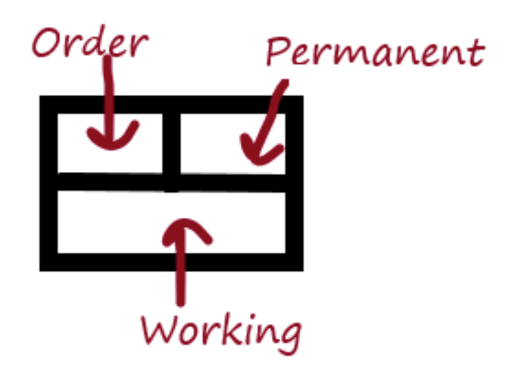
Now, in order to find the shortest route from A to E, we will use a system which involves giving all the towns labels. Each label will include an order space, a permanent distance space, and a working distance space. These things won’t make much sense yet, but that’s okay. All will hopefully become clear as we work through the example. The labels will look like this:
Clearly, if we are trying to get from A to E, then we begin at A, which means that its order number is 1 i.e. it is the first label we complete, with permanent distance 0, since we obviously don’t have to travel any distance to get from A to A. The working distance box will be empty, since we have not had to do any working out here. So our diagram will be updated:
Next, we must work out the distance from A to all the adjacent nodes; that is, all the places we may reach directly from A. In this example, this is B and C. We will write these distances in the working distance boxes for B and C, since we don’t know yet if they are the shortest distances from A.

From here, we can see that it is less distance to reach B than it is to reach C. Dijkstra’s algorithm tells us that this means 10km is the shortest distance from A to B through any route – can you see why? Therefore, we may fill in the permanent distance box for B, and give it order 2, since it is the second town which has been given a permanent distance.

Now, as we did before with A, we will look at all the towns directly connected to town B. As you can see, these are towns C and D. Since town D is 5km away from B, we can put 15 in the working box for D, as we add the distances from A to B, and then from B to D. Remember, we want to know the shortest route starting from A to E.
However, for C, you might notice that there is already a number in the working box! In order to decide whether to relabel this, we must work out what the distance from A to C is via B. This turns out to be 15km, which is smaller than 20km, and so we replace the 20 with 15 in the working box, since we are looking to minimise all distances from A. It turns out to be quicker to go from A to B to C than from A directly to C.

Again, Dijkstra’s algorithm tells us to make the town with the smallest working number permanent, since this must be the shortest possible way to get there from A. But C and D have the same working number! For convenience, I will choose C, since it follows in the alphabet, but you could just as easily have chosen D next. It will make no difference to the overall result.
Since C is going to be our third permanent town, we put 3 in the order box. The permanent distance becomes 15, as this is the smallest number in the working box.

Can you remember what we do after we make a town permanent? That’s right. We look to see the distance from it to any town directly connected. In this case, C is directly connected to D and E. Clearly, there is no point travelling from C to D: we have travelled 15km to get to C, and it would take 10 more to get to D, but we already know that we can reach D in 15km using a different route (as signified in the working box). So we do nothing to D.
On the other hand, we have not put anything in the label belonging to E yet. In order to get from C to E, we need to travel a further 5km. So the number which goes in the working box of E is 20: 15km from A to C, and 5km from C to E.

What’s the next step? We need to make one of the two remaining towns permanent. Have a look at the working boxes of D and E, and try guessing which one it will be.

It was D! Can you see why? D had 15 in its working box, and E had 20. 15 is smaller than 20, so we pick D. Furthermore, D is the fourth label we have made permanent, and so it gets order number 4.
The only other thing we have to do now is look at the distance from D to E. This is 10km, but since we have already travelled 15km to get to D, we can see this route would mean it takes 25km to get from A to E. But we want the shortest route, and the number in the working box of E tells us we’ve already found a route from A to E which is only 20km! So we don’t change anything about E’s working number. Additionally, since E is now the only label left, we can fill in its permanent details: order 5 and permanent distance 20km.

We’re done! The shortest route from A to E is 20km, and by retracing our steps on the diagram, we can see this route is A to B to C to E. Not the most direct route, and certainly not the one you might have picked without the algorithm! As you can imagine, for more complex networks, the shortest routes would be even harder to spot, so this algorithm provides an excellent way of guaranteeing you’ve found the optimal solution.
In fact, if you look at the permanent distances for all the towns, we can see that Dijkstra gives the shortest route from A to any of the towns on the map. What a useful little tool! Still, you are probably thanking your lucky stars right now that your sat nav is able to do this so you don’t have to, because although it isn’t too tricky once you get the hang of it, this algorithm can quickly become fiddly as you add in more places. On the other hand, you can now feel smug that you at least have a vague inkling of how your sat nav works, and can boast to all your friends that ‘it actually uses a variation of Dijkstra’s algorithm, thank you very much’, solidifying your reputation as either a genius or a know-it-all. Have a good journey!
Exercise
In the example above, we used distance as a way to measure between different locations. Different sat nav settings will lead it to determine routes according to different criteria. I will leave you with an example of a problem which instead considers time taken between places in order to find the quickest route from A to F. Why not grab a pen and paper and have a go at seeing if you can work through the algorithm by yourself?

| A | B | C | D | E | F | |
| A | – | 5 mins | 15 mins | 10 mins | No direct route. | No direct route. |
| B | 5 mins | – | 5 mins | No direct route. | No direct route. | 30 mins |
| C | 15 mins | 5 mins | – | No direct route. | 10 mins | No direct route. |
| D | 10 mins | No direct route. | No direct route. | – | 10 mins | No direct route. |
| E | No direct route. | No direct route. | 10 mins | 10 mins | – | 10 mins |
| F | No direct route. | 30 mins | No direct route. | No direct route. | 10 mins | – |
[Scroll down for the solution!]
.
.
.
.
.
.
.
.
.
.
.
.
Solution:

| Order | Permanent Time | Working Time | |
| A | 1 | 0 mins | – |
| B | 2 | 5 mins | 5 mins |
| C | 3 (or 4) | 10 mins | 15 mins, 10 mins |
| D | 4 (or 3) | 10 mins | 10 mins |
| E | 5 | 20 mins | 10 mins |
| F | 6 | 30 mins | 35 mins, 30 mins |
Quickest time from A to F: 30 mins
Quickest route from A to F: A to B to C to E to F OR A to D to E to F
If you enjoyed this article, and want to explore the previous stages of the journey, be sure to check out parts 1 and 2:

[…] Mathematical Holiday Part 3 – Using The Sat Nav […]
LikeLike
[…] Mathematical Holiday Part 3 – Using The Sat Nav […]
LikeLike