
James Somper
Last time, we discussed vaguely what is meant by mathematical chaos, and explored some systems that exhibit the properties required to be classified as chaotic. In this article, we will delve deeper into the chaotic realm and look at what exactly must be true for a system to be chaotic, as well as introducing the logistic map as an example of how simple models can sometimes end up being incredibly complicated.
Edward Lorenz defined chaos as follows: “When the present determines the future, but the approximate present does not approximately determine the future”. There is no universally accepted mathematical definition for what chaos is, but for a system to be considered chaotic, it is typical that three conditions must be satisfied. These conditions were first formulated by Robert Devaney. The three conditions are that the system must:
- Be sensitive to initial conditions
- Be topologically transitive
- Have dense periodic orbits
What is interesting about this definition of chaos is that nowhere in the requirements is randomness found. A system can be perfectly well-defined, with all of its properties being determined absolutely, and yet the evolution of those properties in time can still be chaotic. This is sometimes referred to as deterministic chaos, although since many chaotic systems are inherently deterministic, this is often just referred to as chaos in the more general sense.
The concept of deterministic chaos is summed up well by Lorenz’s quote above: the present tells us exactly how the future will pan out. The system is hence deterministic, as there is no randomness in the future – it depends exclusively on how the system currently exists. However, as the system is chaotic, and therefore has the first property of being very sensitive to initial conditions, the second part of his statement comes to bear, where the approximate present does not define the future well at all. This also links to the overall idea of mathematical chaos being that small changes in initial conditions lead to massive changes in output. This means that if there is any small error in the specification of the initial conditions, this can massively change the final state that is predicted. There is always some error in one’s measurements of physical systems, and so for systems that are chaotic, this leads to the inaccuracies exemplified in things such as weather forecasts.
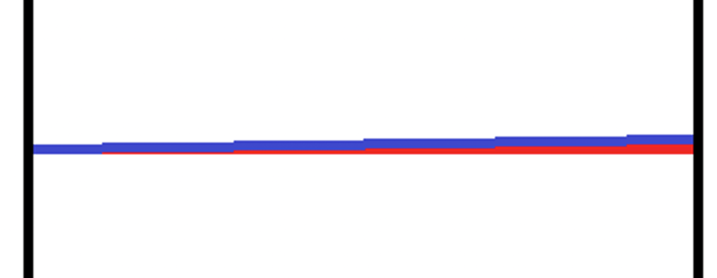
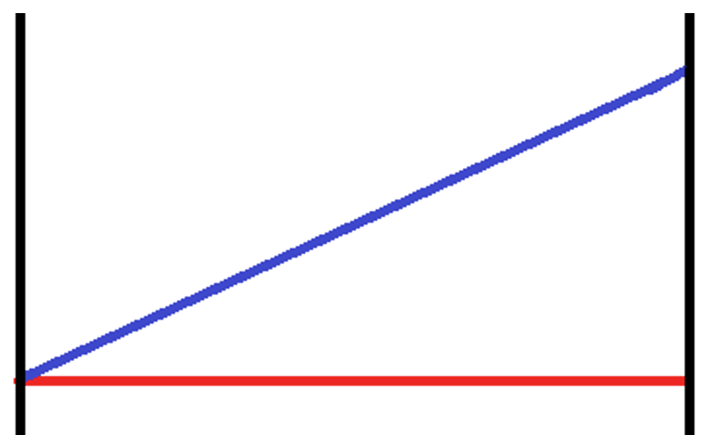
To give an example of how small changes to initial conditions can lead to large changes in the output, let us consider two ships travelling from a port. One ship travels in a straight line, whilst the other one travels in the same direction, but the ship’s captain has made a small error, and has set off at an angle 1° different to the first ship.
From trigonometry, the distance between the end point of these two ships is given by:
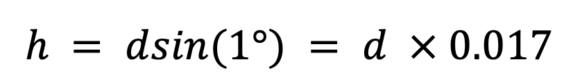
This means that there is around a 2% difference in where the two ships final location. This isn’t a huge difference if the distance travelled is small. However, over distances of 100 kilometres, the two ships are now separated by 1.7 kilometres, which is over a mile away from one another, even though the second ship only started with a change in direction of 1°!
Chaotic systems exhibit a similar sensitivity towards these changes, except the difference can be much larger, and not necessarily scale with the size of the change made to the initial conditions.
For example, if one makes a change of around 1% to the starting values and receives a change that is proportional to that 1% change, then the system isn’t chaotic, as it isn’t especially sensitive to the initial conditions. However, if one makes the same change to a chaotic system, it would be highly likely that the change in the output would be on the order of 10, 100 or even 1000%. Alternatively, it could cause a system that once converged to a value (that is to say, eventually reached a stable value) to now diverge (to not do that). That is the nature of the first condition for chaos.
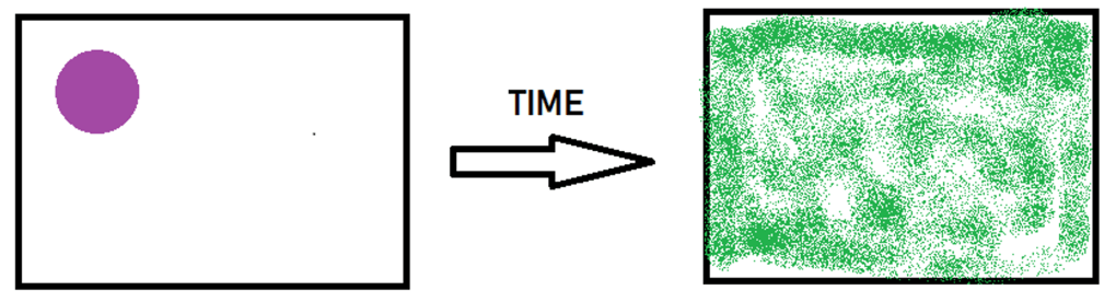
The second condition for chaos is that the system is “topologically transitive”. This is a more rigorous, and stronger form of topological mixing. However, topological mixing allows one to understand what is meant by this stronger condition. Topological mixing describes the phenomenon that, given a fixed set of points, any set of points one chooses in a chaotic system will eventually evolve to overlap with any other set of points. In effect, if one plots the evolution of the system, the page becomes opaque, because all values that can be taken are transformed back and forth between one another (see figure 3 below).
This is an important condition in defining chaos, as a system where the rule for generating the next value is to double the current one is also very sensitive to the initial conditions, but all values eventually tend to positive or negative infinity, and so the system is not inherently chaotic.
The third and final condition for chaos is that the system has dense periodic orbits. This is to say that every single point in the chaotic system is approached (but never reached) by a periodic orbit. A periodic orbit is described by a closed set of values that repeat themselves over and over again. For example, a system that allows input values of 1 to 4, with the rules:
- If current value does not equal 4, then add one
- If current value equals 4, the next value is 1
is an example of a periodic orbit. For chaos, these orbits never reach the initial value ever again, but they can reach arbitrarily close to these values. For example, if the system starts with the value of 1, for the system to be chaotic, there must exist a sequence that brings the system ever closer to the initial value, but never reaches it, no matter how long one leaves the system to run. For dense periodic orbits, this must be true for all points in the system.

We now return to the diagram that was shown last time. This is called the logistic map, and shows a very well-studied chaotic system. The map actually results from mapping a model for population growth. It maps the results that the recurrence relation
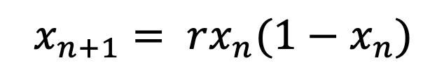
gives, as r is varied. This is a very simple model for population growth, as it contains two terms, one that causes the system to grow, whilst having one term that causes the system to shrink. These can be rationalised as follows: the population should grow proportionally to the current population, as the current population can reproduce. Meanwhile, the population should decrease depending on the amount of resources in an environment, as the environment can only support so many people / animals. Hence there is an extinction factor of 1 minus the current population. Investigation of this system leads to a number of interesting behaviours. Firstly, for all values of r less than 1, the population eventually dies out (that is to say, tends to 0), independent of the initial population, as the new value is necessarily less than the current value. For values of r between 1 and 2, the series converges to a value of:
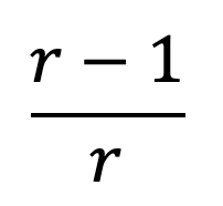
which is also independent of the initial population. Between the values of 2 and 3 the population also converges to the above value, independent of the initial population. However, the value oscillates around this final value, only converging slowly. For r=3 in particular this process takes a surprisingly long time.
The really interesting behaviour – especially for our purposes of studying chaos – occurs for r > 3. Here, the population no longer tends to a value, but instead tends towards a permanent oscillation between two values. This is interesting behaviour in itself, but it is not yet chaotic. The values that the system oscillates between are given by:
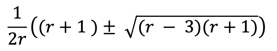
This behaviour continues until a value of r = 3.44949 is reached, where the function then oscillates between 4 values. As r increases up to 3.54409, the oscillations double, first to 8 values, then to 16, then to 32 etc. This is referred to as a period doubling bifurcation, as the number of iterations for the function to return the same value (that is to say, the period) doubles. This is the first indication that the system is beginning to become chaotic, but we aren’t there yet.
The onset of chaotic behaviour appears above 3.54409, with nearly all initial values diverging once r is greater than 4. This is shown on the logistic map by how the region past r = 4 seems almost completely shaded in. This shows that the values rapidly diverge, as well as showing the sensitivity to the initial conditions – a slight change in this value of r sends the function spiralling off on a completely different divergent path. This behaviour is true mathematical chaos, and the general state of the system cannot be easily predicted.
Perhaps most interestingly for the logistic map, we can clearly see regions past these values that are white, and not fully shaded. These are regions where the function assumes semi-stability, and can be interpreted either as a return to convergence, or an oscillation between a number of values. These islands of stability further emphasis the confusing characteristics of chaos, as the location of the islands themselves is equally unpredictable.
Overall, the logistic map provides a wonderful example of how chaos propagates, with such a seemingly simple model proving to be unworkable – for large enough r there simply isn’t a way to easily calculate what will occur. Instead, one must resort to heavy computational methods, which whilst an improvement on pen and paper, are of course themselves still limited by the unpredictability of chaotic systems (see forecast, weather). So, if someone ever asks you to describe what chaos is, from now on, armed with a pen with sufficient ink, you too can explain it to them in gory detail.
In the next article, we will explore weather forecasting in more detail, and try to answer the forever-asked question as to whether we will ever be able to know if next week will be glorious sunshine, or horrendous rain? Without giving too much away, the related question of every weather forecaster of “will they ever stop making fun of me?” is perhaps more apt. See you there!

[…] Clearly, chaos is an important topic in the universe, and to understand the universe better, we require ways to deal with the inherent chaotic nature of these processes. For that, however, we need to take a deeper dive into what chaos means mathematically, which we shall do in the next article. […]
LikeLike