Ellis McKenzie – commended entry in the 2021 Teddy Rocks Maths Essay Competition

When the cynical narrator of Lord Byron’s (1788-1824) epic satirical poem Don Juan exclaims “truth is always strange; / Stranger than fiction; if it could be told”, they could hardly have expected the phrase they thus coined to be referenced in the title of a mathematical essay hundreds of years later. But in the same way that Lord Byron used his poetry to create a fictional abstraction of the ineffable emotions which govern the human existence, applied mathematicians use their equations to create a fictional language to quantify the ultimately unquantifiable Universe.

At its best, this idealised language yields only good approximations of the future. At its worst (when confronted with “chaotic” systems such as the weather), it is simply unable to provide reasonable approximations of the future beyond a finite time frame. Chaotic systems of equations are so sensitive to perturbations in input values that miniscule imprecisions in these will result in huge inaccuracies in output. The underlying framework behind chaotic systems is Chaos Theory, about which this essay will provide a brief introduction. Chaos Theory is the author’s favourite area of mathematics because it challenges the (all too common) trend amongst mathematicians to denounce the humanities as imprecise because of their reliance on abstract human emotions and qualitative reasoning. Chaos is a timeless reminder both that there is just as much beauty in speculative exploration of the unknown as there is in mathematical rigour, and that there is significant overlap between the two categories.

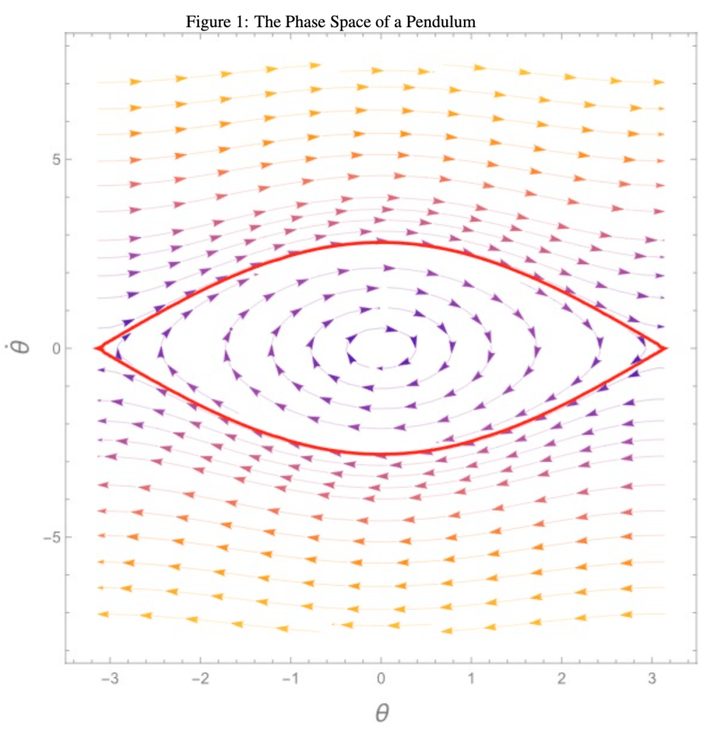
It is first necessary to digress to the non-chaotic world to elucidate some pertinent mathematical jargon. A dynamical system is a system where a function describes how the position of a point in geometrical space varies with the passing of time. Dynamical systems are useful for the modelling of real-world phenomena, such as the oscillation of a pendulum, where an initial point on a Cartesian graph with axes “angular velocity” dθ/dt and “angular position” θ is transformed as time passes. The “phase space” of a dynamical system is a, diagrammatic for the purpose of this essay, representation of all possible states of the system. In the case of a pendulum, it is a diagram of all possible velocity/angular combinations. A certain pendulum’s phase space is shown in Figure 1 .

Figure 1 is a vector field, so each point in the θ, dθ/dt plane is assigned a vector, of which a finite number is represented as arrows. A given starting point on the plot (representing the pendulum’s initial conditions) will be transformed by the magnitude (ranging from yellow (low) to blue (high)) and directionality of the vector on which it lies, and this process will continue continually, resulting in smooth motion. It is clear that starting points within the bold red line (the “separatrix”) will spiral inwards until reaching the centre of the plot (in physical terms, the pendulum will gradually lose energy until angular position is 0 (it hangs perpendicular to its support) and angular velocity is 0 (it is stationary)). Starting points outside the separatrix represent initial states which cause the pendulum to swing in a circular motion around its support, but even these will eventually be “attracted” into a spiral similar to that displayed around the origin. We call the points to which all inputs tend “fixed point attractors”.

Now that we have explored a non-chaotic phase space attractor, we can contrast this with the phase space attractor of a chaotic system of equations. Take the “Lorenz Equations”, a set of non-linear differential equations formulated by Edward Lorenz (1917-2008) as follows:

dx/dt = σ(y−x) (1)

dy/dt = x(ρ−z)−y (2)

dz/dt = xy−βz (3)

These equations provide a simplified model of atmospheric convection. Convection is a type of heat transfer in a fluid (liquid or gas). The equations model a two-dimensional chamber of fluid heated from below and cooled from above; warmer regions towards the base of the chamber will rise because they are less dense than their surroundings, and cooler (denser) regions towards the top of the layer will continually sink below these, creating “rolls” of convecting gas.

The equations describe how the rotational speed of convection (x), horizontal temperature gradient (y) and vertical temperature gradient (z) vary in the chamber with respect to time. By using our simplified definition of a chaotic system (that small changes of input values result in large changes in output values), we can informally prove the Lorenz equations to be chaotic for certain input values. File1 is an audio representation of two solutions of the Lorenz equations, with initial condition x differing by just 0.1s^-1. It is initially impossible to distinguish between the two audio pulses. In this period, a reasonable approximation of the future state of the atmosphere could be made, without fear of measuring imprecisions skewing results. However, after a short while, the audio pulses diverge dramatically: this is the sound of chaos!

File1 was generated using my own Python script which uses the scipy library (specifically the ‘odeint’ command) to numerically integrate the equations at 0.01 second intervals between 0 and 100. The product x × y × z at each time step is passed to pysinewave, which uses it to determine which pitch to smoothly modulate to next.

It can be challenging to understand why this dynamical system exhibits such unruly behaviour. One way of rationalising it is by considering another physical system which it models: the “Malkus Waterwheel”. This is a symmetrical, circular water wheel with buckets filled above from a steady stream of water and with holes in their bases so that water can continually flow out. dx/dt represents the rate of change of the wheel’s angular velocity. dy/dt and dz/dt correspond to the difference in water volumes between the right and left/top and bottom halves of the wheel. At high enough rates of water inflow, the wheel will move sufficiently fast that buckets don’t have enough time to fill up completely before moving downwards or empty completely before moving upwards, causing the spin to slow down and change direction. Aperiodic oscillations between states of acceleration, deceleration and directionality reversal will ensue, in a pattern which demonstrates very sensitive dependence on initial conditions.

Figure 2 shows the phase space attractor of the Lorenz Equations for inputs ρ = 28.0, σ = 10.0, β = 8.0/3.0. An initial starting point (1.0,1.0,1.0) is transformed in the x,y,z plane by three-dimensional vectors corresponding to the solutions to x, y and z over 100 seconds. From these plots, we can infer several characteristics about chaotic dynamical systems. Firstly, two starting points close to each other on the attractor will be rapidly transformed to be arbitrarily far apart, as suggested by the zoomed in plot. This is what causes the above-mentioned sensitivity on initial conditions. The term ”butterfly effect” has now entered the public vernacular to describe any situation where a small action ripples out to have large ramifications, but was coined by Lorenz to describe the sensitive dependence on initial conditions exhibited by this set of equations.

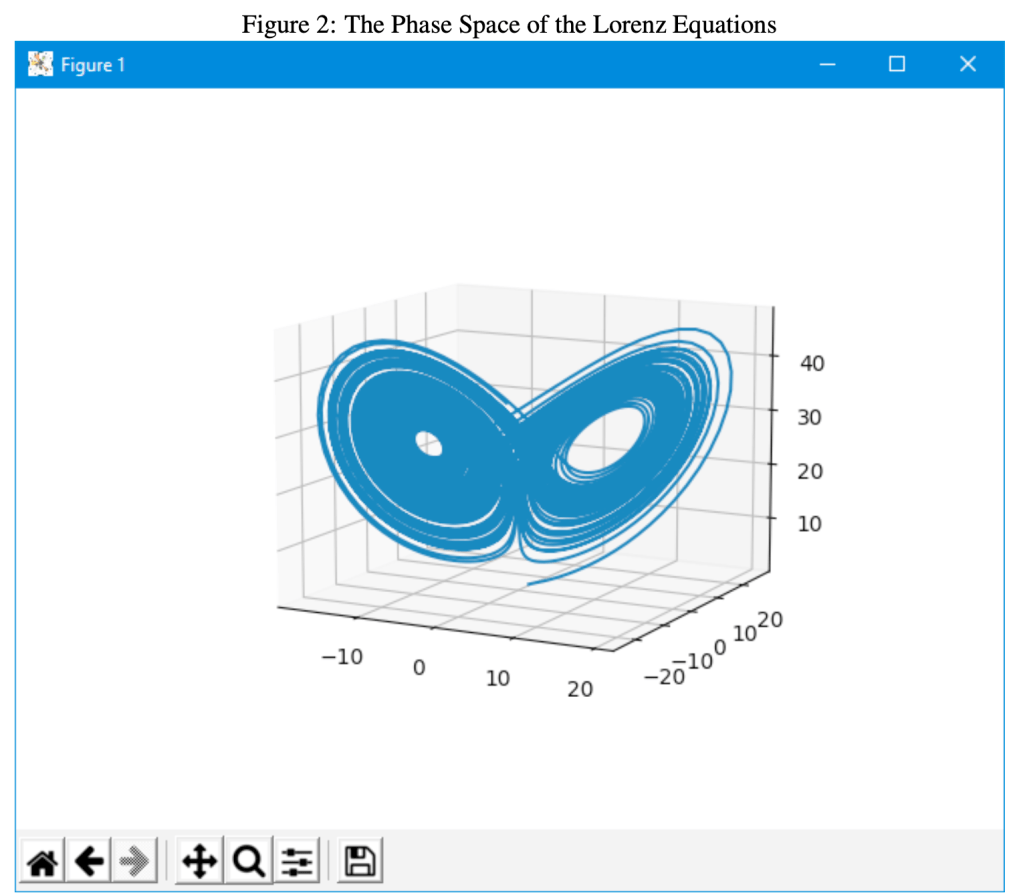
Secondly, the trajectory never branches, so chaotic dynamical systems must be ”deterministic”: there is no random (”stochastic”) element in how the initial inputs are transformed over time. Thirdly, the trajectory never crosses itself (this is unclear in Figure 2 since a three-dimensional graph is being plotted in two-dimensional space), so the equations must be aperiodic; they do not settle into a loop of values in the long term. From these three features, we can finally formulate a definition of Chaos – infinitely aperiodic behaviour in a deterministic dynamical system which exhibits sensitive dependence on initial conditions.

To progress our discussion of the Lorenz Equations further, we should consider what geometric shape would be created if their attractor were generated over an infinite timescale. The resulting shape would have an infinite surface area. However, it would also have a volume of 0 because of the constraint that its trajectory can never cross or merge with itself. In fact, the shape would be classed as a fractal, a type of complex geometrical shape with a “fractional dimension”, an opaque concept discussed in more detail below. A phase space attractor which is a fractal is known as a “strange attractor”, and strange attractors generally (but not exclusively) arise in the phase spaces of chaotic dynamical systems. This is because both chaotic systems and fractals are infinitely, but deterministically, complex.

In defining the concept of the fractal from first principles, it is necessary to consider a new formula for dimension, which yields both the expected Euclidean (integer) dimension for ordinary shapes and a fractional value indicative of the complexity of fractals. Imagine that a shape is broken into identical, self-similar components. The ratio between the width of each of the new subdivisions and the original shape is represented by s. The number of the new subdivisions needed to cover the original shape is represented by n. We find that dimension, D, is yielded from the following formula:

D = log(n) / log(1/s)

First let us apply this to a cube of dimension 1 × 1 × 1 subdivided into cubes of width 0.5, so that s = 0.5 = 0.5. Intuition tells us that eight of these smaller cubes will be needed to fill the original cube, so n = 8. log(8) / log(1/0.5) = 3, so the cube is three-dimensional. Applying this method to a chaotic phase space attractor is well beyond the scope of this paper, but we can apply it to a known fractal such as the Koch Curve to prove that certain shapes have fractional dimensions (including the coastline of Great Britain!) due to their immense complexity.

The Koch Curve (first published by Helge von Koch (1870-1924)) is created by generating an equilateral triangle, drawing equilateral triangles on the middle two-thirds of each of the straight line segments, and then infinitely repeating this latter step, as demonstrated in Figure 3. Per iteration, each of the straight line segments is split into four straight line components, so n = 4. However, each of these segments have a length of one third that of the original line, so s = 1/3. log(4) / log(1/(1/3)) = 1.262, so the Koch Curve has fractional dimension; it is a fractal.

Truth is always stranger than fiction. The study of chaos theory is an important reminder that the natural world is ever more complex than humankind would infer from its innate belief in the doctrine of determinism and their faith in intuition.

Nature is strange. Some physical systems are so sensitive as to be unpredictable beyond a certain time frame. The fractals which their phase space attractors produce cannot be described by the familiar dimensions governing our daily lives. But only when humans choose to stop fearing this “strangeness”, and learn the importance of exploring the unknown, can real societal progress be made.