
Aditi Chegu – Teddy Rocks Maths Essay Competition 2022 Commended Entry
In 2016, Google created “Quick, Draw!” A game that required their neural network to guess the subject of its players’ drawings. I always found how the game learned to guess what dragons were from over 50 million drawings of subjects ranging from arms to animal migration incredibly fascinating.
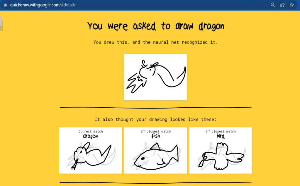
Similar to our brains, neural networks take inputs, and send certain reactions to neurons in the network. Neural networks are made up of layers of neurons. The neurons in different layers are connected by “weights”, a parameter that defines how the input should be transformed. Each neuron also has a “bias” which determines the threshold past which a neuron should be activated. The information of inputs passes through the layers of the network after which a final prediction is given. Which, in this case, was that my drawing was of a dragon.
When a neural network is first created, it has no information about the task at hand. So, it assigns arbitrary values to all the weights and biases. Due to this random assignment of values and lack of training, the output of the network for a given task is usually rubbish. But, much like students learn from their mistakes and correct what they do wrong, neural networks can also improve in their performance by tweaking their weights and biases to provide more accurate results.
To improve the neural network’s performance, we have to first assign a value to the quality of its performance. This value should quantify the error between the expected prediction and actual prediction for a training example– essentially, it is the “loss” of the neural network for that particular training example. For example, if given a drawing of a dragon, a bad neural network might return a 0.4 probability for the image being that of a dragon and a 0.3 probability each for it being a fish or a bird. To quantify this inaccuracy, the loss can be written as the sum of the squares of the differences between the probability expected and actual probability.

After the neural network is given sufficient training data, a collection of all the different losses can be gathered. These losses show how poorly a network is performing for specific examples given their parameters– weights and biases. So, the average of all these losses would express the performance of the network as a whole. A high loss means that the network is inaccurate, whereas a low loss means that the network is accurate. To improve the accuracy of the network, the losses need to be minimised.
Because we know that the losses are dependent on weights and biases, we can use them to help us reduce the loss. To do this, we start by defining some function which returns the average loss when all the values of the weights and biases are taken as inputs. Then, we have to change the values of these parameters to minimize the loss as much as possible.
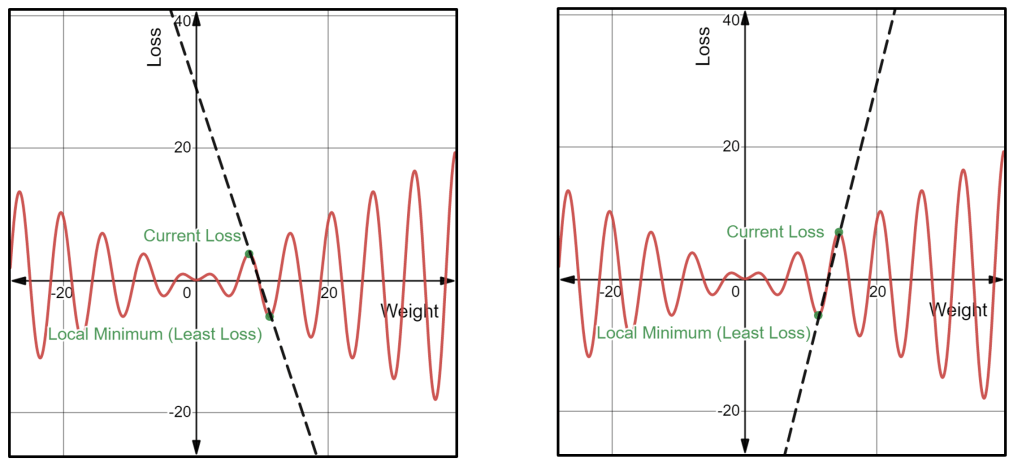
For example, if we take only one parameter as the input– weight– and one output– loss– the loss function represents the change in loss with respect to a change in the weight. In this graph, loss is graphed on the y-axis, and weight is graphed on the x-axis.
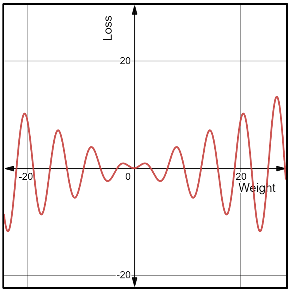
We are at a certain point on this loss function depending on the arbitrary weight assigned, and to minimize loss, the point should be moved closer to its local minimum. To move the point downwards, we need to know the direction and magnitude by which it should be moved. This can be done by taking the gradient of the function at that particular point. If the gradient is negative, then the point can be moved further to the right to find a local minimum. Similarly, if the gradient is positive, the point can be moved further to the left to find a local minimum. This process for finding the local minimum of the loss function is called “gradient descent”.
In this example, there is only one input that varies the average loss. In reality, however, millions of inputs influence the average loss. This means that graphing them, with all the parameters having one axis each and the output having another axis too, would mean having a graph with millions of dimensions– which is inconvenient, to say the least. However, the process of gradient descent can still be executed by using some clever calculus.
As previously stated, each parameter in the loss function needs to be changed in some way to edge towards the least possible loss. To do this, we need to find the direction and magnitude by which the parameter needs to be changed.
Loss functions often have millions of parameters (variables) as inputs, so, to find the direction and magnitude of change for one parameter: we have to take the derivative of the loss function with respect to that one parameter while keeping all the others constant. By doing this, we are finding the “partial derivatives” of the loss function.
Done manually, calculating all the partial derivatives would be equivalent to a death sentence. Even if we use a computer to find these values, the fact that we are using the processes of differentiation that we learn in high school calculus– manual differentiation– will quickly fail us.
An elegant way of making this less cumbersome is by exploiting the fact that differentiation can be an extremely mechanical process once the basic rules are set in place.
For this, the loss function is deconstructed to give its constituent operations and functions. This deconstruction can be represented as a “computational graph” where all the nodes represent operations (+, -, /, *) and functions (sine, cosine, log) and the edges show how the nodes are related.
The process is made of two phases: forward pass and backward pass. In forward pass, the function’s inputs are entered into the graph to evaluate their values. In the backward pass, it uses the chain rule to piece the function back together by calculating the derivatives at each node.
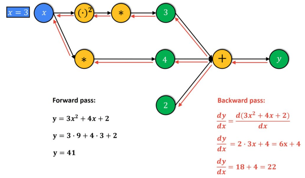
By using this method, “automatic differentiation”, we can calculate the exact partial derivatives independent of the size of the input, unlike all the other processes of differentiation (numeric, symbolic, manual).
Equipped with the partial derivatives, we now know the gradients of each parameter. Parameters with higher gradients can cause huge decreases in cost with small changes, and parameters with smaller gradients cause small decreases in cost with small changes. Making the appropriate adjustments to the weights and biases will therefore result in a reduced cost function and an increase in accuracy.
As we can calculate the magnitude and gradient descent required with greater computational and mathematical efficiency, the neural network becomes better at distinguishing dragons from all the other drawings with greater certainty much faster.
This process through which Google’s neural network learns and improves is implemented in all neural networks– from improving text to speech transcription, to sorting data, to generating Gmail’s automatic responses– mathematics models the world around us and improves our ability to cope with it too.
Sources:
https://towardsdatascience.com/
https://mostafa-samir.github.io/auto-diff-pt1/
https://marksaroufim.medium.com/automatic-differentiation-step-by-step-24240f97a6e6
https://towardsdatascience.com/automatic-differentiation-explained-b4ba8e60c2ad

Thank you teacher I’m taking my flight test my teacher ordered me to marry Rory he is also British
获取 Outlook for iOShttps://aka.ms/o0ukef
LikeLike