Ifan Rogers

A traffic jam on the motorway is an all too familiar sight for many of us, whether it’s being surrounded in a car full of siblings, or stuck in a bus with no air conditioning. Often after inching forwards bit by bit, we find that the traffic starts moving again and the traffic jam magically disappears… It turns out that all it takes to form these ‘phantom traffic jams’ is for one vehicle to slow down. A slight change in speed of one car causes the one behind it to decelerate, and the same for the vehicle behind that and so on. And what we end up with is a ‘shock wave’ of cars starting and stopping that travels up the motorway against the direction of traffic.

Mathematically, we can model this as a longitudinal wave, where vibrations travel in the same direction that the wave is moving. We can illustrate this with a slinky – the popular toy which has found its way to every physics classroom for all time. When the slinky is briefly compressed on one end, we see the packet of compression propagating to the other end (as shown in the animation below). This is already similar to how a traffic jam ‘shock wave’ can travel up the motorway, we simply replace coils of a slinky with cars.

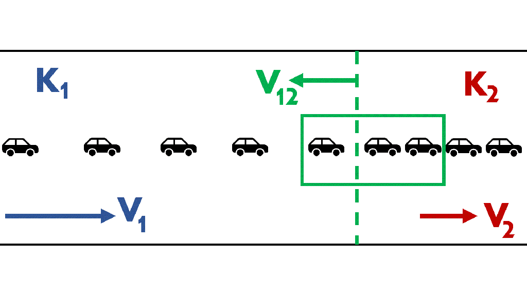
The next question we might want to ask is how fast does this shock wave travel up the motorway? To do this we need to zoom in on the boundary where free (uncongested) traffic becomes part of the traffic jam, let’s call these regions 1 (the left edge) and 2 (the right edge) respectfully. For each region we associate a vehicle density (measured in numbers of vehicles per km), denoted by K and a speed at which all vehicles travel at, which we’ll call V. As the vehicle density increases, which means more cars on the road, the speed of each individual car must decrease.

We see the boundary between regions 1 and 2 travels backwards, just as we expected from our slinky model. This moving boundary makes our calculations awkward, so we will employ a common trick physicists use, we will move with the boundary such that it remains stationary with respect to us.

We can see an example of this effect on the motorway as follows: if 2 cars travel at the same speed, then each car seems stationary with respect to the other one. Of course, to a burger van in a lay-by, both cars are definitely not stationary, they’re whizzing past at great speed. The situation from the perspective of a moving observer is what physicists commonly refer to as a ‘reference frame’.

We’ve added our new reference frame below in green – notice how the line separating the two regions remains stationary inside this box which simplifies the calculation.

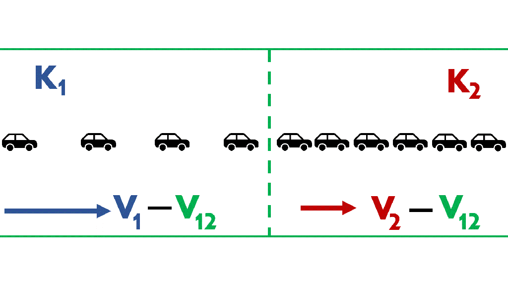
Our next task is to make this reference frame stationary, which we do by allowing everything else to move backwards with the shock wave speed, V₁₂. This means we need to subtract the shock wave speed from the velocities in regions 1 and 2. The animation below shows the green box, now stationary, zoomed in.

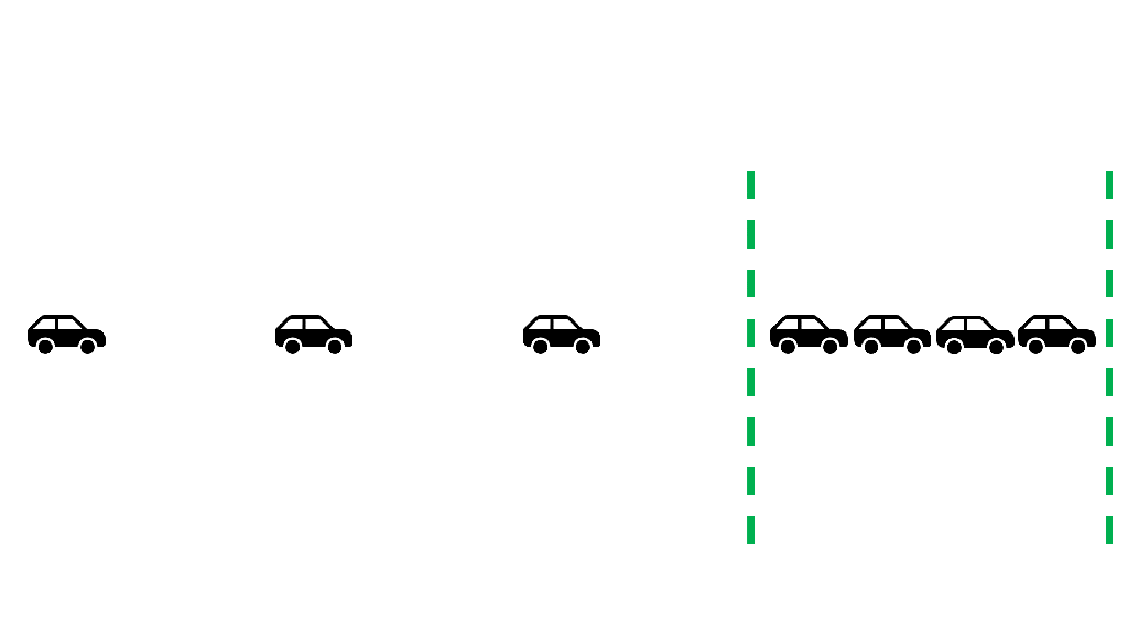
All that’s left to do now is to apply ‘conservation of cars’ across this boundary. Cars cannot be appearing and disappearing from the motorway, so any car leaving region 1 must arrive in region 2. Multiplying the density and speed of a region gives us the number of cars leaving or arriving in that region. We’ll call this the vehicle flux and denote it by Q. By equating the flux on both sides of the boundary, we arrive at an expression for the shock wave speed.

Next, we are going to explore how the vehicle flux varies with the density. As with most modelling problems, let’s start by looking at the limiting cases when the density is 0 or at a maximum value of K_max. For the first case, a density of 0 corresponds to no cars on the road, and so the number of cars arriving/leaving the road is 0. While at a maximum density, all the cars are in a traffic jam, and so no cars can arrive or leave, meaning the flux for this case is also 0. Many functions satisfy this, but to find the exact one we consider the propeties of the road such as the number of lanes, the visibility and the road condition. As an example, let’s use a general concave function between our two points.

We can now go one step further and represent the speed of the shock wave on this diagram. Firstly, we identify where on the curve regions 1 and 2 are and we connect the two points with a straight line. The speed of the shock wave between these two regions is represented by the gradient of this line. If the vehicle flux decreases from region 1 to 2, the gradient between them will be negative which corresponds to a backwards travelling wave. Conversely, if the vehicle flux increases, the gradient would be positive and the traffic shock wave will travel forward, with the traffic.

So, what happens on the motorway? After the first car starts braking, a compressed region of cars is formed, where the vehicle density is much higher, but the flux is lower. This creates two boundaries on either side of the compressed region. One where the density increases but the flux decreases, and another where the density decreases and the flux increases. Going back to the diagrams above, we see the gradient in both of these cases are negative, causing both boundaries to travel against the direction of traffic. The effect of this is a compression packet travelling up the motorway, just like what we saw with the slinky.

So the next time you’re stuck in a frustrating traffic jam, just remember you might be in the compressed part of a motorway-long slinky made of cars. And hopefully, you’ll start moving again soon.