
Congratulations to Jed Skilling for their essay entitled “The Undeserved Mystery of Complex Numbers” – the Student Winner of the 2023 Teddy Rocks Maths Essay Competition.
“Jed’s essay is an excellent example of how to introduce an advanced topic to a non-specialist audience whilst also showcasing a novel way to think about complex numbers. I found it very easy to follow, highly intuitive, and thoroughly enjoyable – well done!”
“From [Grothendieck], I have also learned not to take glory in the difficulty of a proof: difficulty means we have not understood. The idea is to be able to paint a landscape in which the proof is obvious.”
Pierre Deligne
1 Introduction
The definition of an imaginary number is most commonly one of two things:
√ i = −1
i2 = −1
And just looking at this, surely one must ask “Why?”, what’s the benefit of this seemingly paradoxical definition; we’ve all been told since primary school a number multiplied by itself is positive. So how can we define something like this and why is it useful?
I would like to answer both these questions, despite the extravagant (and rather vague) name, I don’t think complex numbers should be treated as some new and frightening field of maths, but rather a beautiful addition and a powerful tool to use.
2 Laying the groundwork
When we run into a new problem, or find ourselves in new mathematical circumstances, one of the first steps we should take is, surprisingly, backwards.
For example, instead of trying to tackle the new problem, think about any simpler examples you may already have seen. Have you seen a problem or ideas similar to this before? Could you solve a simplified version?
By looking at a simpler case, we can analyse the key ideas and methods we can use to solve the more complex problem in front of us.
For instance, if you had to plan a revision schedule for your final exami- nations, you might look back at how you revised for individual examinations. What were the key themes and ideas you focused on? Has anything changed since then? Did your system work well?
2.1 Rediscovering Negative numbers
In this case we may look at how negative numbers were introduced to the mathematical world. For such a common thing, which now seems inseparable from modern mathematics and everyday life, they are actually quite abstract.
I start the year with an unknown count of seeds, and by the end of the year, I have harvested 4 times the number of seeds as I planted (assuming I plant all of my seeds), and in December, a friend also donates me 20 seeds. If I now have 4 seeds, how many did I start with?
If we let the seed count be x, we can formulate the equation: 4x + 20 = 4, and rearrange to get 4x = −16, and therefore x = −4. But this doesn’t make sense, as I cannot start the year with a negative number of seeds.
Indeed, this is what led the 3rd Century Greek Mathematician Diophantus to declare the equation 4x + 20 = 4 as absurd.
So if negative numbers are so abstract, how do we think about them?
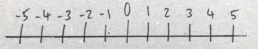
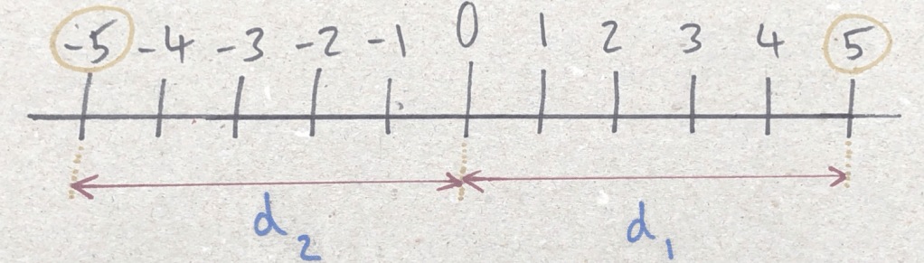
The answer is that we would use a number line, but how does that let us separate the negatives and the positives? What makes -5 different from +5? They both lie the same distance from 0; it is their different direction which distinguishes them.
What we can see is that every number has a certain value, and a measure of its direction from our origin of zero.
Although the distance d1 = d2, +5 and −5 are not the same due to their different direction relative to our origin.
2.2 Generalising
We have now introduced a new idea to our regular number system, direction, two numbers can have the same distance from the origin, but in a different direction, giving you two distinct numbers.
Now, we should look at how we can generalise and formalise our discovery. What does direction mean? Can we assign it a value? What can we do by changing a number’s direction? How else can we use this?
One way of measuring direction, is by treating it as an angle.
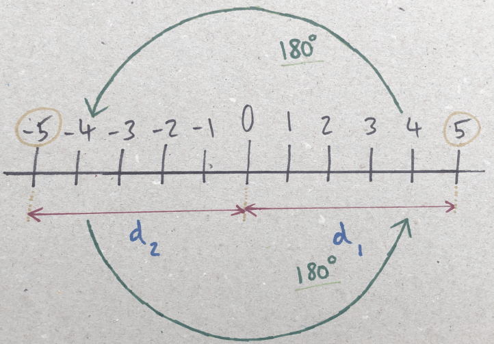
Figure 3: Direction as an angle
As we can see the “angle” for the positive number is either 0 or 360*, and negative numbers are 180, notation wise, this will be denoted (by convention) to be the argument, denoted by arg(x), where x is our number.
*We denote positive numbers as having an angle of 0 or 360, as you can get to positive numbers in two ways, rotating by 0 degrees, in effect staying in the positive numbers, or by making a full rotation of 360 degrees to move round our whole number line. Rotations beyond 360 just loop back to 0.
When “dealing with distance from the origin” we calculate it with the modulus or absolute function |x|, which is just a more compact way of referring to the distance of x from the origin, we will be denoting this value as the magnitude of our number.
3. What do we do next?
Some examples of our new operations are shown below:
Modulus:
|−5| = 5
|2| = 2
Argument:
arg(−4) = 180
arg(4) = 0 or 360
Now we have some more concrete ideas we have come up with, we can start playing around with them. Is there a pattern we can see? What happens to the magnitude of a number when you multiply two of them? What about the angle?
I’d encourage you to explore this further, try multiplying a few numbers together and seeing what happens.
A simple thing we may notice, is that magnitude remains independent from argument; if two numbers multiply together to give a number with a magnitude of 10, changing either of the number’s argument (making them negative or positive) will have no effect.
|−5 × 5| = |5 × 5| = 25
A similar, (though maybe less obvious) pattern is that the same holds for the argument; the product of two numbers will have the same argument no matter what magnitude you pick for the initial numbers.
arg(5 × −5) = arg(7 × −8) = 180
3.1 New arithmetic
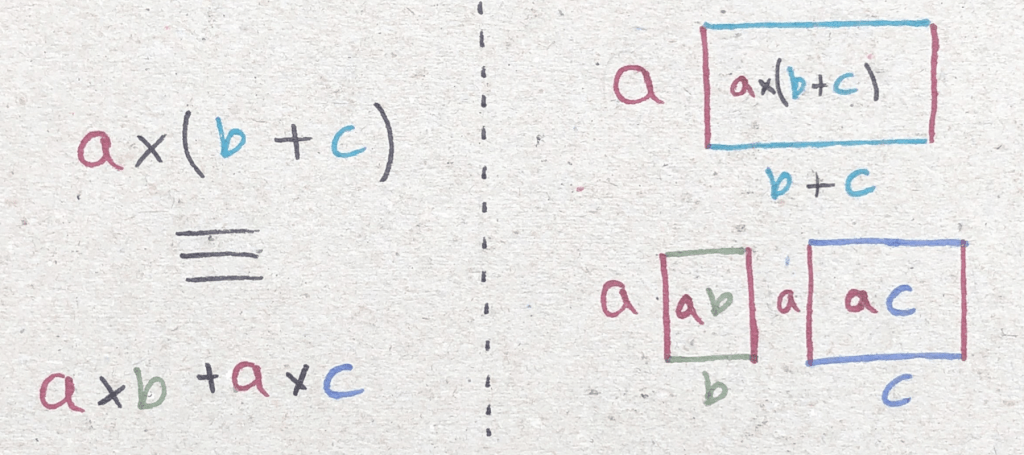
From exploring along with pattern spotting, you may notice that the magnitude of the product (multiple) of two numbers, is the same as the two magnitudes of the individual numbers multiplied together. Stated mathematically this is:
|a×b| ≡ |a|×|b|
The ≡ just means that this is always true, no matter what values of a and b you choose.
This property is known as distributivity, and is also shown by multiplication, as shown here, with the mathematical and geometric interpretation side by side:
Looking at the argument function under a similar lens, we can note that the multiplication rule does not hold, −1 × 1 = −1, whereas multiplying the arguments will give us an angle of 0 or 360. The 360 comes from the fact that a positive number has an angle of 0 or 360, due to being a full rotation round our circle, or no rotation at all.
Instead, we may see that the arguments aren’t being multiplied, but have a different combination, see if you can spot the pattern! We will be denoting the unknown operator as *.
1×1=1
0 * 0 = 0
1 × −1 = −1
0 * 180 = 180
−1 × −1 = 1
180 * 180 = 360 or 0
Though it may not be immediately obvious, our mystery symbol, *, for multiplication is just addition! When we multiply two numbers, we just rotate the first number by the argument of the second number. This is why two negatives give us a positive, the two half rotations return our angle to zero (180 + 180 = 360), and this puts us among the positive numbers.
4 Squaring and Square rooting
The next section brings us to the penultimate step before we can introduce the imaginary number in all its glory, and I do encourage you to make sure you fully understand all the previous steps; you need a strong understanding of the functions and properties we have learnt for this final jump.
I will be focusing on how the argument changes here, as it is ultimately more interesting than the magnitude for the purpose of introducing complex numbers.
4.1 Squaring
So, here we are, we now have our idea of angle and magnitude, and how changing them affects our original number. Now we have formulated and experimented with the simple cases we should move to consider more complicated cases.
1) Do our rules hold for squaring? 2) Square rooting? 3) What patterns are there is these results? I hope to show in this section how these three questions are very interconnected.
If we let n be a random positive or negative number, what will the argument (angle) of n2 be?
To put this in a familiar context, we can write this out as n × n, which allows us to apply our previous knowledge, that multiplying two numbers, changes their arguments by adding them together and therefore simply doubles the angle.
If n is negative, we have two negatives 180 + 180 = 360, therefore arg(n2) = 360 or 0. And for positive n the angle is either 0, therefore the new argument is 0 + 0 = 0 or 2 × 0 = 0, or 360, therefore giving an angle of 360 + 360 = 720 or 2 × 360 = 720.
Make sure you remember any angle above 360, like 720, is just going to be multiple full rotations, so we can, and often do, interchange it for 0 or 360. Visually, if you pick something up, and rotate it through a full 720, (two full rotations), it will return to its original orientation.
4.2 Square rooting
Square rooting a number is effectively the inverse of squaring. If we square root a number, we expect to get a number that, when squared, returns us our original number.
Defining our arguments for square rooting may seem complicated at first, after all, the square root of a positive number is multiple things, both 2 and -2 go to 4 when squared, so how will we address this when square rooting?
Both −2 and 2 equal 4 when squared: (−2)2 = 22 = 4
This implies both 2 and -2 are the square roots of 4:
√4 = ±2
The first thing to notice is that we will need to inverse whatever changes we have made when we squared our original number.
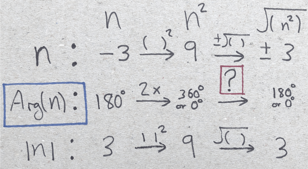
To reverse our change of doubling the argument, all we do to the angle is half it! If we replace the question mark with: 12 × or ÷2, we can see that to get from 360◦ to 180◦ we have divided by 2.
But then where does our ± symbol come from?
The answer to this question lies in how we treat a full rotation (or zero rotation) as being both 0 and 360.
Because our angle of 360 is both 360, and 0, when we divide by 2, we do not have enough information to choose one value. Therefore, we use the ± sign to show that we cannot say for sure which value it was. We can state our new rules for the argument mathematically as:
Arg(n2) = 2 × Arg(n)
Arg(√n) = 1/2 × Arg(n)
And now, we are finally ready for the last step.
5 The final leap
5.1 Magnitude and Angle Form
We now have before us all the tools to make the final step and introduce the complex number. By defining the square root in terms of its effect on the magnitude and the argument, we have expanded its input.
By our usual definition of the square root we cannot give an answer to this equation:
x = √ -1
This is because we are restricted to arguments or angles of 0 or 180, and we cannot find a number to satisfy both of these constraints at the same time.
However, we have expanded our definition of the square root, and we can work out the expected magnitude and argument we would get:
|√n| ≡ √|n|
arg(√n) ≡ 1/2 × arg(n)
And if we plug our equation x = √−1 we can get values for the modulus and argument. Try it yourself!
x = √−1
|x| = √|−1|
|x| = √1
|x| = 1
arg(x) = 1/2 × arg(−1)
arg(x) = 1/2 × 180 = 90
Therefore, as our final result we get:
|x| = 1
arg(x) = 90
Although it may seem strange to get an angle that isn’t 0 or 180, there is nothing mathematically wrong with this answer. What the means is that it satisfies our equations, and is consistent with our old rules. If we were to go in the reverse, i.e. doubling the argument and squaring the modulus, we would get back to -1; we haven’t broken any rules of mathematics.
I would recommend experimenting with this a little bit. Try testing out what multiplying our new number by a positive does, or a negative. See what happens when you multiply √-1 by other values.
5.2 Cleaning this all up
Although this is all mathematically sound, it has started to become a bit cum- bersome. You can see why we just use a negative sign to represent negatives rather than listing out their angle and magnitude, or learning the argument rules, etc. For most purposes this is fine, it is faster and more convenient to work with. What we want to do now is apply those same time saving methods to what we have developed here.
So therefore, how can we make our system more convenient for a wider range of angles?
For this, we return to our old friend the number line again. Though imperfect at the moment, we can improve upon it.
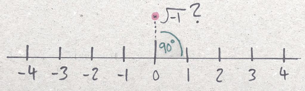
Although looking like some strange mutation of the Number Line at first, the position of √−1 makes sense. Angles of zero are to the right of the origin, angles of 180° are to the left of the origin. This leads on naturally, to angles of 90 being directly above the origin. Shortly, we will look at how we can use this to create a grid structure to express any number more complex than just a positive or a negative.
Notes on notation:
From now on I will be denoting any number with an angle that is not either 0 or 180, as being a complex number, or in notation, as n ∈ C, where C is the set, or collection of all complex numbers, and ∈ just means n is in C.
So, we know that an argument of 90, (and a magnitude of 1) will give us a value of √-1, but what about 45? 270? 134? Well if we look at the diagram below;
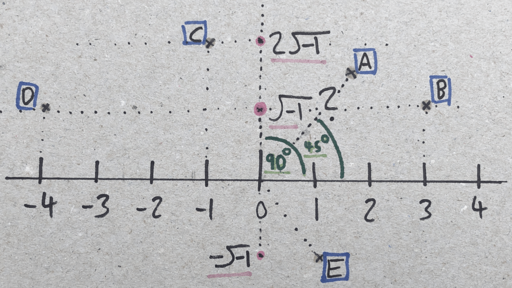
We may notice that A could be described not by an angle and a distance, but instead by its horizontal and vertical distance from the origin. The horizontal distance refers to what we call the Real section, and can be denoted as a coordinate x, where x ∈ R, which just means x is a number that is on our old and boring number line and can only have positive or negative values.
For the sake of faster notation, and distinguishing complex numbers from real numbers, mathematicians avoid using √-1. They manage this by substituting in the arbitrarily chosen letter i. Instead of writing √−1 we can instead write i, thus we define i as:
i = √−1
What previously seemed like some arbitrary choice, has now been simplified away; merely a nice trick to speed up writing.
We can do the same with the vertical value, we will call it y, and this tells us how high up it is, or what the −1 is scaled by (we can see that 2√−1is higher up than √−1, 2i > i). Here, y refers to the scaling factor, so it is also a real number (y ∈ R).
We can see some examples of this notation below (as usual try and predict and guess along). In calculation we often switch between the angle-magnitude form and the x and y method; both have their advantages and disadvantages.
√−1 ⇒ x=0, y=1
2√−1 ⇒ x=0, y=2
arg(z) = 45, |z| = √2 ⇒ x=1, y=1
i ⇒ x=0, y=1
1 ⇒ x=1, y=0
With our new co-ordinate system, we can write any complex number z (so: z ∈ C), as being made up of those two coordinates, effectively:
z = x + iy
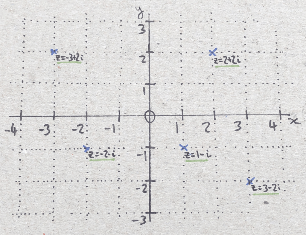
And thus, we can now state any complex number we want.
6 Conclusions
I hope my essay has not just taught you about a new (or your first!) way of look- ing at complex numbers, but also a wonderful (and in my view) beautiful way of looking at new problems, via a rigorous series of simplifying, identifying key patterns and generalising. I believe many seemingly unobtainable problems can be addressed, using methods like this, and not only in maths! Providing motivation and problem solving with new topics ourselves can be a great experience, and it truly is a shame we often don’t have time for this in education.
If you want to look more into the wonderful results we can get from using the complex plane, I would recommend looking at some functions or operations we already know, and trying to introduce complex inputs. There are so many more beautiful aspects of the complex world I wish I had time to at least mention.
But now that baton lies in your hands; so go run with it!

[…] 2023 Overall Winner: Georgia Skiada2023 Student Winner: Jed Skilling […]
LikeLike