Agnieszka Wierzchucka

In everyday life, if you want to find the position and momentum of an object, it’s pretty straightforward. Let’s consider the example of a car. To find its speed, and therefore momentum, we can use a speedometer and a scale. Then to find its position, we can simply open Google maps. The obviousness of such a property in our everyday life makes it hard to accept that in the realm of the very small, i.e. the quantum world, this isn’t always the case. In fact, the so-called ‘uncertainty principle’ says that such a simultaneous measurement is actually impossible – if we know the location of an object, we cannot also know its momentum (and vice versa). Such a profound statement might seem like something straight out of a sci-fi film, but over this series of articles I plan to discuss the maths behind it, and try my best to give you some sort of physical intuition as to why it exists.

As with most physical statements, in order to understand it, we must first set out on a quest to learn the required maths. We will start with a little bit of algebra, or more precisely vectors. You will likely have come across the idea of a vector before – an object with a length and direction. You might have even have seen them in column form. However, there is a more general definition of a vector as an object which satisfies a set of rules, not too dissimilar to how a shape is a rectangle if it has two parallel sides. Using this more general definition, functions can be thought of as vectors, as can states of a coin flip: heads/tails. (In fact, we will come back to the idea of these so-called ‘state vectors’ in the last article.) There are seven rules in total which define a vector, but we won’t focus on their exact statements today. (However, if you are curious, do look them up here – you might be surprised how simple, yet powerful they are.)

We begin by defining a ‘space’ of vectors as a set of vectors that satisfy some property. For example, all vectors of the form (a,b,c), or all the functions which describe a straight line. We can combine vectors and their multiples together to make more vectors, like so:

Here, we add the vectors component-wise, so the first entry of 7 is the result of adding 1 and 2 times 3 together. Check that you are happy where the other two entries come from.

Now of course, some vectors are more special than others. We call a set of vectors independent if none of the vectors can be made out of the others. For example, the above three vectors, (1,0,2), (3,1,1), and (7,2,3), are not independent as we can make (7,2,3) out of the other two – add the first one to two times the second one. However, the standard unit vectors, (1,0,0), (0,1,0), and (0,0,1), are, since it is not possible to make any of them using combinations of the other two.

Another idea which we will need on our quest to understand uncertainty is the idea of a ‘Basis’. If you have a space of vectors, its basis is a special set of independent vectors such that every vector in the entire space can be made up from combinations of the basis vectors. You might find it helpful to think of a basis as the bricks that build up the vector space. As an example, the aforementioned standard unit vectors make a basis for 3D space. But (1,1,1) and (2,2,2) don’t as there is no way to make (0,1,0) out of them.

The last concept we will need at this stage is a linear function, sometimes called a linear operator. You have likely come across these before, even if you don’t recognise the name. A function can be thought of as a machine that takes an input vector, does something to it, and then outputs the result – kind of like a kitchen robot taking in an apple and spitting out an apple pie. In life, there are many different machines. One might make an apple pie, but another might make a fruit salad. A linear function is a machine that behaves in a certain way. One very important property of a linear function is that putting in the sum of vectors to the machine is the same as putting the two vectors in separately and then adding the output. Also, putting in a vector times a scalar gives the same output as putting in a vector and then multiplying the output by that scalar. This may sound a little abstract so let’s look at an example:

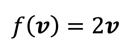
This is a linear function as if we take two vectors, v and w, and a scalar “a”:

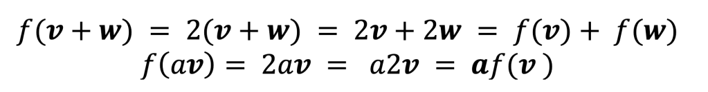
So, the function f(v) = 2v satisfies all of the rules for a linear function.

However, g(v) = |v| is not a linear function, as if we take -1 and the vector v = (3, 0, 4):

But:

So, the function cannot be linear as it doesn’t satisfy the second (and in fact also the first – check this for yourself!) requirement for linear functions.

Ok – phew! I’ll forgive you for thinking we are moving further and further away from the uncertainty principle, but I assure you this will all be very useful later… In fact, we are now about halfway through our trip to the quantum realm. Make sure you’ve followed everything we’ve discussed so far as in the next article we’ll be moving on to talk about matrices. See you there!