
Agnieszka Wierzchucka
So far on our journey to understanding the uncertainty principle we have explored the concept of vectors and linear maps (see part I). Our next and last stop before getting to the world of quantum is the matrix – well not the matrix but matrices in general…
Unlike the popular sci-fi film, a matrix is an array of numbers. It is made up of rows and columns and can have any size, where the entries can be real or complex numbers. (If you don’t know what complex numbers are this article is a great way to learn about them.) The idea of matrices might seem very elementary, as, after all, they are basically an overcomplicated grid. However, matrices are extremely important objects in maths. They are the building blocks of transformations (e.g. rotations and reflections), cryptography, and as we will soon realise, quantum theory.
The vectors we were discussing in the first article are examples of matrices, just small ones with only one column. General matrices, however, do have their own special behaviours. For example, we can only add them if they have the same size, and if they do, we just add the respective entries, exactly as we do with vectors. Multiplication of matrices is a little more complicated, but don’t worry we’re going to go through an example below. And I will just stress at this point that this might seem very random – it certainly did to me the first time I came across it – but stick with me as it is essential to get us to where we want to go.

Instead of multiplying element by element, matrix multiplication works in a “row-by-column way”, as shown above. We start with the first row of the left matrix and the first column of the right matrix and multiply the individual elements (blue). Then we do the same but with the second column instead of the first (orange). We repeat this process with the second row of the left matrix (green and red) to get the final matrix product. If the matrix is larger than in this example, the process is extended in the same way.
This method of multiplying matrices means that it is not always possible to find a product of two matrices – the left matrix has to have the same number of columns as the number of rows in the right matrix. If this isn’t the case, then, like trying to put two wrong puzzle pieces together, the multiplication won’t work. This might come as a surprise as we are not used to such a feature with our more familiar numbers. Another consequence of this rather odd way of multiplying matrices together is that the product of two matrices might not be the same if the order is reversed, i.e. AxB might not equal BxA. As you will see in the next article, this can in fact be interpreted as the reason why the uncertainty principle exists. Provided both matrix products exist, we use a commutator, AxB – BxA, to assign a value to how much the two orders of multiplication ‘disagree’. The most useful matrices are square ones, as they are nice and simple to work with, so we will mostly focus on them from this point onwards.
Ok, so why are these little glorified grids relevant to our previous discussions? Well, the fun part of matrices is that any linear function can be written as a matrix – matrices just provide a different way to display the function, which is useful in certain situations. Consider the map from the first article f(v) = 2v, where v is a 2D column vector. Below you can see it represented by the matrix:

Let’s make sure it works by trying it out on two vectors, and following the procedure for matrix multiplication outlined above. We multiply the first row of the left matrix by the first column of the right matrix (the vector), but as there is only one column (blue), this means we are done here. We then repeat this for the second row of the right matrix (orange) to complete the calculation.
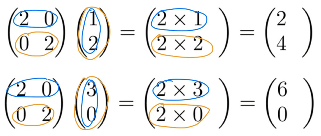
You’ll hopefully note that the output in both cases is exactly twice the input vector, as defined by the function. So, as we’ve seen in the above example, matrices can be a very useful tool if you have complicated linear maps, as they provide a cute and compact way to express them.
The real stars of this matrix discussion, however, are eigenvectors, and each matrix will have at least one of them. When a matrix acts on an eigenvector all it does is multiply it by some value, which we call an eigenvalue. However, it’s important to note that this doesn’t mean the matrix does this to every vector, or that every matrix does it to the same vector. The particular vector that corresponds to an eigenvalue is called an eigenvector, and they are really sort of special. From our above discussion of the f(v) = 2v map, we can see that every 2D vector is in fact an eigenvector with eigenvalue 2, since multiplying by the matrix just multiples every vector by 2.
Now, you might be thinking that the maths topics I have presented in these two articles seem quite arbitrary, and their link to quantum mechanics isn’t obvious. But, I am happy to inform you that after this short algebra course, we are finally ready to talk about the uncertainty principle – coming up in the third and final article – see you there!

[…] an electron. For example, we can make it more likely the electron is found in the 1st box. In the second article, we mentioned linear maps can be represented by matrices, and that these matrices have special […]
LikeLike
[…] to the quantum realm. Make sure you’ve followed everything we’ve discussed so far as in the next article we’ll be moving on to talk about matrices. See you […]
LikeLike