
Agnieszka Wierzchucka
Quantum mechanics is one of the most important theories ever created by humankind. It is unlike any area of physics you have seen before, so don’t worry if it all sounds like a sci-fi movie. One of the fathers of the theory, the Danish physicist Niels Bohr actually said that if you don’t find it confusing, you don’t understand it. The uncertainty principle, which we will now explore, is just one example of the many weird phenomena quantum mechanics implies.
Unlike in the macroscopic world, the quantum realm is ruled by probability. In particular, it uses “probability amplitudes”, so the probability of an event occurring is given by its probability amplitude squared. The need for probability exists due to the fact that measurements on the quantum scale don’t have fixed values – the most we can know is the probability of a specific measurement. It’s like throwing a dice. You don’t know what value a given throw will give, but you can assign a probability to each value it could be. This is the reason why so many people found quantum mechanics hard to accept – they had to let go of the notion that everything has a fixed, defined value. To demonstrate these ideas, let’s consider an example of an electron moving around two boxes:
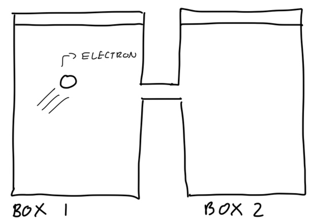
Now at any point in time, the electron is in one of two states: it’s in box 1 or in box 2. To find out which state the electron is currently in, we look inside the two boxes. We are being physicists here, and so we can assume the electron is never in the middle section when we check the boxes. As I mentioned in the first article, these states can be thought of as vectors v1 and v2. When we open the boxes, the electron has a clear, definite location, but when they are closed it can be in any of the two boxes. A probability can be assigned (and so a probability amplitude) to the electron being in each of the two states when we open the box: A1 is the probability amplitude it is in the first box and A2 is the amplitude it is in the 2nd box. Then a state vector, let’s call it w, can be created which encodes all this information: w = A1v1 + A2v2. Any electron zooming around between the two boxes can be described by such a state vector, so we can think of v1 and v2 as a basis for the states of the electrons (check article 1 for a reminder of what a ‘basis’ is if needed).
We can extend this “box example” to the positions of an electron more generally. Again, consider an electron moving around. At any point, an electron is at some position x, which we assign to the state vector vx. Then each state has a corresponding probability amplitude, let’s call it Ax, so Ax2 is the probability the electron has position x when we measure it. Then a state vector can be written that describes this particular electron, but this time in terms of its position: w = sum of Axvx for all the possible positions the electron can have.
As the electron is not standing still, this whole process can be repeated, but with the possible values of momentum, p of the electron. So, we can write : w = sum of Apvp for all the possible momenta. Every electron must have some sort of momentum and position when we measure it, so vx and vp form two bases for these electron properties, which means every electron can be described by how likely it is to have particular positions/momenta.
Unsurprisingly, we can repeat this with many properties of the electron. These quantities (position, energy, box number etc.) are called observables. So, as you can see, the state vector w encodes all the information you can have about the electron. You can think of it as a fact file, from which we extract information by writing it in terms of the components of specific basis vectors.
As w is a vector, we can act on it by linear operators to change the state of an electron. For example, we can make it more likely the electron is found in the 1st box. In the second article, we mentioned linear maps can be represented by matrices, and that these matrices have special vectors called eigenvectors. Out of all the linear maps that can act as the state vectors, two are very important to the discussion of the uncertainty principle. Let’s first focus on the ominous sounding “position operator” X. Fortunately, it is actually a lot simpler than it sounds. When applied tow, all it does is multiply all the Ax values by the corresponding value. For example, if the electron had only two possible positionsx = 3 and x = 4:
w = A3v3 + A4v4 and Xw = 3A3 + 4A4v4
This specific operator has eigenvectors vx with eigenvalues x. There is an identical operator corresponding to the momentum called, (surprise, surprise) the “Momentum Operator” P, which has eigenvectors vp with eigenvalues p. This acts differently to the position operator and is very similar to taking the derivative of a function d/dx (see BONUS below for more information).
Putting all of this together we have:
Xvx = xvx and Pvp = pvp
These operators might seem very arbitrary, but they are actually very powerful concepts we use to make some sort of sense of the quantum world.
Now, imagine we want the probability of firstly measuring the momentum to be p and then the position to be x. Nothing says this has to always be the same as the probability of measuring the momentum to be p and then the position to be x (ie. changing the order of the measurement). As a result, when we measure quantities of an electron, they might depend on the order we measure them in. In fact, the only time the order wouldn’t matter is if XP = PX (which means the operators are commutative).
*BONUS: If you want to check this is indeed the case, try applying the XP and then PX to the state x and see what happens…
PX(x) = P(x2) = d/dx (x2) = 2x
while XP(x) = X d/dx(x) = X(1) = x
A famous physicist, Werner Heisenberg proved this isn’t the case – the position and momentum operators are NOT commutative. From this we can deduce that we cannot know the momentum and position of the electron at the same time. As if we could, we would get the same result no matter the order we measure its position and momentum. This is the uncertainty principle – the impossibility of being simultaneously certain of an object’s position and momentum.
Well, this sure was a long and eye-opening journey through quantum mechanics. I hope I managed to achieve the goal I set out to complete and it gave you more of an idea of why the uncertainty principle exists. Heisenberg was just one of many involved in the quantum revolution, so this principle is the only the peak of the iceberg of quantum systems. Now I need to go and ask a man about a certain cat that may be both simultaneously dead and alive…
If you want to learn more about Heisenberg’s Uncertainty Principle you can watch Tom explain the mathematics behind it to fellow YouTuber Michael Penn here.

[…] algebra course, we are finally ready to talk about the uncertainty principle – coming up in the third and final article – see you […]
LikeLike