Vlad Bercovici

You may have seen the most recent match-day graphics for the Premier League and noticed a quirky new thing “powered by Oracle” describing the win probability of each team. Maybe you wanted to place a bet on the latest US Open match and checked the odds of each player beforehand. Perhaps you flipped a coin, rolled 2 dice at once, or played Rock-Paper-Scissors with your friend, praying that you’d get tails, or 2 sixes, or that your buddy picks scissors. At the very least, you may have uttered a phrase such as “What are the chances?” or even seen a meme along the lines of “Every event has 50% chances of happening: it either does, or it doesn’t”.

Even in the unlikely event that nothing in the list above applies to you, what matters is what they have in common: the concept of probability. It makes its presence felt at all times, and in some aspects it even guides our lives. But what is this probability thing exactly? And why has it been studied so intensively by mathematicians for almost 5 centuries? 

Consider an event in the future, any event. Will Chelsea win the league this year? Will you be given homework to do next Thursday? Answering such questions constitutes a prediction, a belief that something will happen. Probability is a quantifier of how strong that belief is, a numerical description of how likely that prediction is to come true and of the corresponding event to occur. The mathematical probability assigned to an event is a number from 0 to 1 (which is why we often see it described as a percentage from 0% to 100%), such that 0 means impossibility and 1 indicates absolute certainty. Furthermore, as you may have guessed, the higher a probability is assigned to an event, the more likely it is to happen.

Of course, with events in the past, or those based on scientific facts (e.g. sunrise and sunset) it is very easy to assign a probability, either 0 or 1. However, the future is usually filled with many variables, inconsistencies and what-if’s. Probability can extinguish some of the fear about upcoming events, providing a sense of certainty in our world of uncertainties. With the correct mathematical theory applied, it can serve as an objective predicting tool for the price of stock, the quantity of wool sheared in Scotland, the number of cases of HIV next year, and so on…

However, it is dangerous to interpret probability as more than a simple measurement of likelihood and to take the numbers assigned to an event as acts of clairvoyance, especially if they are very close to either 0 or 1. No matter how many experts tell you to buy Tesla stock, a single catastrophe can make its value drop faster than a barrel down the Niagara Falls. While probability is a very useful tool to make somewhat informed and reasonable decisions, it should be treated with the utmost care as, in some cases, mathematics cannot replace instinct. Such examples of “defying the odds” can be seen in stock trading, with the famous GME saga, or in sports, with the well-known case of Leicester City winning the Premier League despite bookmaker odds of 5000-1.

An extreme example of how probability can be so beautiful, yet so fragile was spotted in American football, more specifically in Super Bowl 51, the game to determine the winner of the NFL between the Atlanta Falcons and the New England Patriots.

The Falcons, shown at the bottom-left of the graph, were leading 28-3 in the middle of the 3rd quarter; in terms of actual football, it roughly translates to winning 4-0 with about 20 mins to go. At that point, the win probability for Atlanta was so dangerously close to 100% (it quite literally intersects with the x-axis of the graph), that if anyone had only seen this portion of the graph without knowing the events, they’d all predict an easy win for them. Here’s the second portion of the graph:

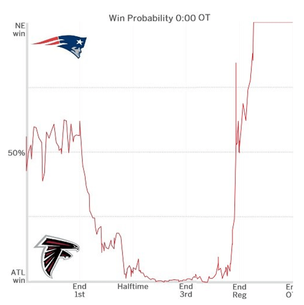
In the end, the Patriots (upper part of the graph) mounted an incredible comeback to win 34-28 and lift the trophy. In doing so, they defied their very minuscule win probability and seemingly maths itself. What on Earth happened?

Well, simply put, Atlanta choked. It isn’t what happened on the field that matters to us though, but the squiggly line that the win probability took as it swung completely from one side of the graph to the other. It started at a certain point before the match, with New England having the slight edge, and it fluctuated wildly as the game progressed. Each event on the field, be it a touchdown, an interception, or an injury to a key player, altered the belief of what was going to happen, and thus the confidence in predicting a winner. As a result, the win probability changed constantly, until the Falcons snatched defeat from the jaws of victory. The idea that the probability of an event depends a lot on other events and does not simply remain constant until it happens is also captured by mathematical theory. Namely by the concept of ‘conditional probability’. For 2 events A and B, the conditional probability of A happening given B has already happened is represented by the following formula (which only makes sense if the event B has a non-zero chance of happening):

As you might have guessed, P(event) is the notation used for the numerical probability of an event occurring, e.g. P(Arsenal win the Premiership this season) = 0. The event referenced in the numerator is that both A and B occur, as suggested by the intersection sign. Thus the conditional probability “of A given B” depends on both events happening (simultaneously or one after another), but also on the second event actually occurring in the first place.

Many events in real life are inter-related; Ford stock depends on the market performance of the company, as well as on rivals such as Chevrolet. To win the Premier League, Liverpool need the results of 19 other teams to go their way (including matches against them). This is why understanding how events condition one another and, more importantly, which events actually influence something else is essential, regardless of what the butterfly effect might tell you. Of course, if two events are clearly independent of one another, then the probability of “A given B” is just the probability of A, since the event B does not influence it; the second dice roll is never affected by the first, regardless of any superstitions.

More impressively, one can reconstruct the original probability of an event using entirely the events on which it depends. This is known as the ‘law of total probability’ or the ‘partition theorem’. The second name is given because the events on which we “condition” have to form a partition, namely to constitute all possible events that can happen…in some sense. For example, all the results of a football match, of tossing a coin or rolling a die can be a partition. The formula for an event A and a “partition” of events {B1,B2,…} is

The formula can be understood as follows: since the Bi’s form a partition, only one of them can happen at a certain time step (you can’t get heads AND tails at the same time), so whenever the event A happens, exactly one of these events will also occur. Adding them up is a natural consequence of considering all possible cases.

For example, suppose that you play a simple game where you roll a fair dice twice and you win if the sum of your rolls beats a certain randomised score. The RNG Gods weren’t too kind, giving you a score of 8 to beat. Using the law of total probability, you can compute beforehand your winning odds by conditioning on what the first roll might give you, so that you know whether it’s worth trying to roll again.

Thus, a partition we can use is the 6 possible outcomes of a die roll; we can denote B_i as the event that we get the number i on the first throw, and A as winning the game. Since both dice are fair, we know that P(B_i)=1/6. Hence the probability of winning turns out to be:

To finish the computation, we simply need to look at the conditional probabilities, and the corresponding events. If the first roll is a 1, you simply cannot win, so P(A|B₁)=0. If the first roll is a 2, you can only win if the second roll is a 6, and there are 6 events that can happen after the first roll, namely the outcomes of the second, so P(A|B₂) = 1/6. If the first roll is a 3, you can win with a second roll of at least 5, and there are still exactly 6 total possibilities, so P(A|B₃) = 2/6. Continuing in the same fashion, P(A|B₄) = 3/6, P(A|B₅) = 4/6, P(A|B₆)=5/6, and the winning odds are P(A) = 1/6 * 15/6 = 15/36. (You can verify all these equalities by simply writing down all possible rolls and their sum, then comparing it with 8).

In the end, we cannot talk about probability without at least mentioning betting and gambling. After all, the theory of probability was only developed after a man named Gerolamo Cardano studied the gambling games of his time back in the 16th century. Of all the mathematical theory related to gambling developed since then, a particularly depressing concept sticks out: the gambler’s ruin. It is not just a theoretical idea, but also a topical problem that millions of people in the UK are affected by, as many go against probability to try to secure great riches. In this 3 part series, our aim is to mathematically argue why gambling is much more foolish than it seems, with the gambler’s ruin concept playing a key role.

In the next article we will move on to the seemingly unrelated ‘recurrence relations’, but before doing so, we need to acknowledge once more just how intriguing of a concept probability actually is. The fact that mathematicians, interested in absolute certainty through their pursuit of mathematical proof, have been studying the opposite of what they believe in for 5 centuries is nothing short of incredible. Thanks to their work, we can now make more analytic predictions and decisions. But, as beautiful as it may be, probability is no clairvoyance. No one really knows what will happen in the future (I’m looking at you Atlanta…). So, always make the choice that you will regret the least!

Article 2: Linear recurrence relations and how to solve them