
Vlad Bercovici
Write down a number, any number. Now multiply it by 2, add 3 and write down the result. Now take the number you just wrote, double it again, add 3 and write down the new result. Do this infinitely many times and…congratulations, you defined a sequence using recursion! All you needed was a simple rule (multiply by 2 then add 3), which is formally known as a recurrence relation. But what exactly is a recurrence relation, and how could one “solve” an equation such as xn+1 = 2xn + 3? How can one classify such relations, and, most importantly, how can you use them to compute, say, the 7th term of the sequence you just built?
To answer that, we first need to clarify recursion. Simply put, recursion happens when something is defined in terms of itself or something of the same type. Rather surprisingly, one can observe such a phenomenon without putting pen to paper or pressing a key. This visual recursion is known as the Droste effect, or “picture within a picture”. An image appears recursively within itself, giving the impression of an infinite loop which really only goes as far as the quality can allow.

In mathematics, the most common form of recursion is generating a sequence of numbers (such as the sequence of odd integers). This is done by applying an equation which gives a term as a function of preceding terms in the sequence. Usually it’s nice and it only depends on the previous number, for example xn=xn-1 + 2, but at times it can rely on even earlier terms, such as xn = xn-1 + xn-2 + 17n. Much like Spongebob holding an image in the meme above, each equation represents a rule by which an entire thing can be constructed. This rule is the “recurrence relation”.
A key observation is that, in the Droste effect example, we needed an original image on which to recurse. A mathematical sequence also requires some initial terms to get the recursive ball rolling. These terms are known as “boundary conditions”, and any respectable sequence has at least one such term (usually just one, but there may be more).
Now actually solving recurrence relations can be a dark art, but there is a subclass of these which can be solved rather quickly. That subclass is referred to as “linear” recurrence relations and contains some of the most famous recursive formulas. Any equation where a general term xn (or sometimes xn+1, depending on the convention) is written as a sum of preceding terms, each multiplied by constants that do not change regardless of n (those are known as “constant coefficients”), or multiplied by a function depending on n, can be put into this class. For example xn = (-3)xn-1 + 4n2, xn = xn-1 – 2xn – 3 + 5xn – 4, or the three equations mentioned before in the article are linear. However, relations such as xn =(xn-1)2 + (xn-2)5 or xn = xn-1 xn-4 + xn-2 are not. A sequence (xn) for which the equation is true for any n ≥ 0 is considered a “solution”. It is this type of recurrence relation that we will learn to solve today, starting from the simplest ones: linear recurrence relations of first order.
The reason they are called “first order” is that every term in the sequence, except for the first one, can be written as the same function taking only one input: the previous term. The most common cases are of the type xn+1 = axn + b or xn+1 = axn + bn. It should be pointed out that a cannot be zero, as otherwise you are not defining a recursion, but rather a constant or linear sequence as boring as watching Arteta’s Arsenal play.
The method we will use, which can be generalised to higher orders where more preceding terms are referenced, makes use of homogeneous recurrence relations. In layman’s terms, these are equations containing only the terms of the sequence, each multiplied by constant coefficients; the unattached constant or expression dependent on n is removed (or, better put, is zero). One can see that, for the first order case, the homogeneous linear recurrence relation is xn+1 = axn.
After finding a sequence (un) that “solves” this homogeneous equation, we can find a particular solution (vn) to the initial recurrence relation by continuously “trying the next most complex thing” (constants, then 1st-degree polynomials involving n, then 2nd-degree polynomials involving n and so on), a trick which some may recognise from solving differential equations. Adding the 2 relations up and factorising properly on each side, one can obtain a general solution (xn), such that xn = un + vn for each n ≥ 0. We then only need to plug in the “boundary conditions”; that is, replace xn and vn with the corresponding values to find more information about un. This will be enough to deduce the general term of the solution we actually need.
If this explanation sounds confusing, it will hopefully make sense in practice. As a first application, we will work on the sequence created at the start of the article. The equation mentioned there, xn+1 = 2xn + 3, wasn’t entirely random, since it is the exact mathematical translation of the rule we used: multiply by 2, then add 3. Firstly, we solve the corresponding homogeneous equation, which is un+1 = 2un, using the revolutionary method of… “putting it into itself”:
un = 2un-1 = 2(2un-2) = 22un-2 = … = 2nu0
(Notice that the exponent of the constant coefficient and the index of the term always add up to n: for 21un-1 we get 1 + (n-1) = n, for 22un-2 we have 2 + (n-2) = n, and so on until for 2nu0 we have n + 0 = n).
As we have no useful information available about u0, we will note it down as an unknown constant A (it could be anything), and write the solution of the homogeneous equation as un=2nA.
To find the particular solution (vn), we first look through constants to see if they can provide a solution. Namely, we try vn = C and replace the values conveniently in the original equation, finding either the value of C or a contradiction:
vn+1 = 2vn + 3 becomes
C = 2C + 3, or C – 2C = 3, which gives C = -3.
Hence vn = -3 is a particular solution of the recurrence relation, and the general sequence (xn) thus has the following formula:
xn = un + vn = 2nA – 3
(Knowing that un+1 = 2un, vn+1 = 2vn + 3, you can check that indeed xn+1 = 2xn + 3. You can also check that the first few “general” terms, namely A – 3, 2A – 3, 4A – 3 and so on, obey the rule).
As a “boundary condition”, we can use the first number you wrote down, namely the initial term x0. We will assume that it’s 1 (it probably isn’t, I’m not a clairvoyant), and replace n with 0 and xn with 1 to find A:
1 = 20A – 3, which gives A – 3 = 1, so A = 4.
So the general term for that sequence you wrote down might have been 4*2n – 3 or, if you prefer, 2n+2 – 3. Now instead of writing down 999 numbers to find the 1000th one, you can simply plug n = 1000 into this formula to compute it directly. Amazing!
First order linear recurrence relations have surprising applications in real world finance, as well. Suppose that your friend down the pub opens an investment account with an initial sum of £1000. They tell you their account should grow at a fixed interest rate of 1% per month, and that they add 5 pounds to it at the end of every month. By writing down the recurrence relation xn+1 = (1 + 0.01)xn + 5 (careful: 1% = 0.01) and using the boundary condition x0 = 1000 and the same method as above, you too can compute how deep your buddy’s pockets will be after 36 months, or 3 years. (Spoiler alert: not that much).

We will now take a look at “second order” linear recurrence relations, named so because, as you may have guessed, the terms in the sequence are written as an equation of the 2 preceding terms. Their most common form is xn+1 + axn + bxn-1 = f(n); we will analyse the simpler cases where the right-hand side is a constant. Here both a and b must be non-zero: b since otherwise the relation is just first order, and a because otherwise the rule would be incomplete, skipping every other term and ruining the recursion.
The method applied in the first order case works just fine here, however, finding the homogeneous solution is a bit trickier. We assume that our solution is not a dull as dishwater sequence of 0’s (formally, it’s non-trivial) and just skip straight to taking un = Aλn. We have Aλn+1 + aAλn + bAλn-1 = 0. Each term has a common factor of Aλn-1, so we can rewrite this as Aλn-1(λ2 + aλ + b) = 0. Now, if we divide by Aλn-1 (this is possible, as both A and λ are non-zero), we will finish the derivation of what is known as the “auxiliary equation”: λ2 + aλ + b = 0.
If this derivation proves difficult to memorise, just remember that we can “reach” the auxiliary equation by replacing the terms of the sequence with powers of λ. The quadratic itself is important to remember, however, since in order to find the homogeneous solution we need to solve it and compare the roots, giving us 2 cases:
- The roots λ1 and λ2 are different. Then the homogeneous solution is un = Cλ1n + Dλ2n
- The roots λ1 = λ2 = λ are the same. By “trying the next most complex thing” (just as we did before), we get the homogeneous solution un = (C + nD)λn.
Like Michael Schumacher at the wheel of a Ferrari, these solutions work brilliantly (but you may check if you’re a Hamilton fan). More importantly, you need to compute 2 constants to get your general term; hence you need at least 2 boundary conditions in this case (after all, 3 + 7 and 4 + 6 both give 10, but 3 + 2*7 ≠ 4 + 2*6).
We will now look at a rather artificial example, meant to show the quirks of repeated roots and of the process for finding a particular solution: xn+1 – 2xn + xn-1 = 1. The auxiliary equation is pretty nice here: λ2 – 2λ + 1 = (λ – 1)2 = 0, with repeated root 1. By looking at the scheme above, our homogeneous solution is un = An + B. For the particular solution, we will yet again try things that are as simple as possible. Notice that taking xn as a constant would just cancel the left-hand side out. A 1st-degree linear polynomial already solves the homogeneous equation, so we can ignore it as a component for the particular solution since it cannot contribute (remember: A and B may still be any number). We hence try a 2nd-degree polynomial which means taking vn = Cn2. Substituting in we obtain:
C(n+1)2 – 2Cn2 + C(n-1)2 = 1, which simplifies to 2C = 1 or C = 1/2.
The general solution is hence xn = An + B + 1/2n2. Indeed, you can check the equation and verify that this is the correct solution (we won’t do the computation here, but If you know the rules of squaring and are careful enough, a lot of terms should cancel out nicely).
To finish things off in a beautiful way, we will look at the most famous recurrence relation: Fibonacci. The idea is simple: we write down 1, then 1 again, and every number after that is the sum of the 2 preceding it (1,1,2,3,5,8,13,21, and so on). While cute at the surface, this recursion hides something incredible, which can only be revealed via the methods we have learned thus far.
Firstly, from the rule we can pinpoint the recurrence relation xn+2 = xn+1 + xn, or, in a more useful form, xn+2 – xn+1 – xn = 0, as well as the boundary conditions x0 = x1 = 1. The resulting auxiliary equation, as one can hopefully see, is λ2 – λ – 1 = 0. This is a particular case of the general quadratic formula aλ2 + bλ + c = 0 for a = 1, b = -1, c = -1. b2 – 4ac = 5 > 0, so we have 2 real roots, namely (-b + (b2-4ac)1/2)/2a and (-b + (b2-4ac)1/2)/2a or, in our case, (1 + 51/2)/2 and (1 – 51/2)/2. Notice that both roots are irrational, even though the quadratic has integer coefficients.
While we had more work to do to solve the quadratic, this is where the fun begins, as Anakin Skywalker once said: the relation is already homogeneous. Great, no need to do any more guess work, we can just plug the roots in:
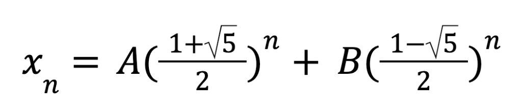
The two initial terms now tell us that A + B = 1, A(1 + 51/2)/2 + B(1 – 51/2)/2 = 1, from where we obtain (by solving the system of equations) that:

Which gives us for any n ≥ 0:

Quite incredibly, an entire sequence of integers is generated only by irrational numbers, even if they have absolutely no overlap! This observation is at the heart of the golden spiral, a geometrical object that at every quarter turn gets wider by a factor of 1 + 51/2, an unfathomable number, but which can be created using squares we can actually draw.

Whether you want to calculate the student loan you will give back to Boris with interest, the exponentially increasing price tag of Kylian Mbappe, or just draw a very attractive spiral, recurrence relations may be there with you. Linear recurrence relations, in particular, can have applications of the most surprising kind, one of which is going to be explored in Part 3 of the series (coming soon), as we dive into a mathematical model of the “Gambler’s ruin”. We hope to see you there!
Article 1: Probability is everywhere. But what is it exactly?

[…] the next article we will move on to the seemingly unrelated ‘recurrence relations’, but before doing so, […]
LikeLike
[…] Despite the well-known health risks associated with gambling, many people around the world still take huge risks and bet their hard-earned money at slot machines and casinos in the hopes of getting rich quick. Perhaps, even when reading the percentages above that are close to 50%, you believed that with just enough luck you could dethrone Jeff Bezos by spending a few days in Nevada. The reality could not be bleaker, and that’s before you even consider concepts such as house edges. The idea that such high percentages can be so misleading just because they are on the wrong side of 50%, is at the basis of the gambler’s ruin, the statistical concept teased in Part 1 of this series, which we will study using the theory we have developed in the second article. […]
LikeLike
So powerful, Stacey, on so many counts. I think foremost is the sharing of your own progression as a teacher of writing- I remember those hamburger organizers! I think of how many students dutifully comply with such things … but what a world of difference there is between compliance/checklists and creativity/real communication. Being shown how to communicate your own thoughts, your own ideas, things that matter to you in a way that impacts others is immeasurable in the spectrum of learning AND LIFE. It’s both craft and creative freedom; parameters are removed vs. enforced. I could go on – just thank you for this labor-of-love post. I have Warner’sWhy They Can’t Write: Killing the Five-Paragraph Essay and Other Necessities and have used it in summer writing pd for teachers at all grade levels; this book is mighty, inspiring, and true. One of my favorites on how to revise the way writing is taught- and empowering tge writer.LikeLike
LikeLike