Vlad Bercovici

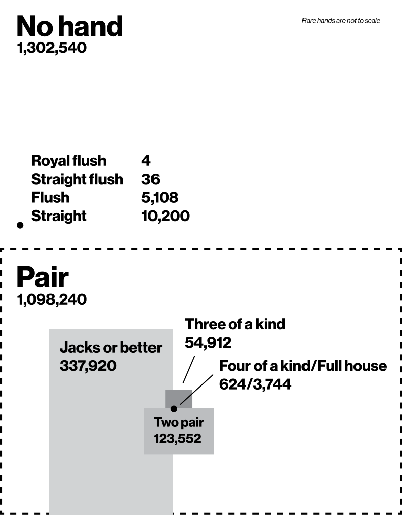
The “safest” bets one can choose when playing European roulette – namely the even/odd, red/black or low/high which cover almost half of the table – each have a probability of 48.6% of returning a profit, dropping to 47.4% in the American version. For a simplistic slot machine with 5 fruits and a Joker, only 44.4% percent of the combinations are winners, with the percentage dropping to around 42% in more sophisticated versions. Even in poker, a game based on psychology as well as pure luck, 49.9% of the hands are winners, although it’s important to note that a large number of those are relatively useless one pairs (42.25% of all hands), leaving a rather measly number that can put up a fight against a human opponent.

Despite the well-known health risks associated with gambling, many people around the world still take huge risks and bet their hard-earned money at slot machines and casinos in the hopes of getting rich quick. Perhaps, even when reading the percentages above that are close to 50%, you believed that with just enough luck you could dethrone Jeff Bezos by spending a few days in Nevada. The reality could not be bleaker, and that’s before you even consider concepts such as house edges. The idea that such high percentages can be so misleading just because they are on the wrong side of 50%, is at the basis of the gambler’s ruin, the statistical concept teased in Part 1 of this series, which we will study using the theory we have developed in the second article.

In fact, one of the more commonly used meanings of “gambler’s ruin” is exactly this: regardless of the betting system a gambler chooses, if the game has a negative expected value then they will eventually go broke. Another common meaning is that a gambler with finite wealth who plays a fair game will inevitably go broke against an adversary of infinite wealth. 

The mathematical model we will use is known as a random walk (sometimes called a drunkard’s walk). This concept describes a succession of random steps around a place where the rules of movement show, for each position, the probability of moving anywhere else and, most importantly, depend only on the current location, not on what was visited before. While you don’t have to learn this definition, it is important to understand the following problem (which was taught to us in the first year Probability course at Oxford as a version of the Gambler’s ruin problem) and its solution, since they lie at the heart of our analysis:

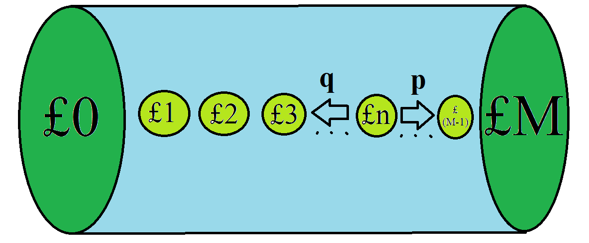
“A persistent gambler repeatedly plays a game in which he wins £1 with probability p and loses £1 with probability 1-p (which we will denote q). Each round he participates in is independent from the others. He will only leave the casino if he loses all his money or if he reaches a fixed fortune £M. Assuming he starts with £n, what is the probability that he goes home broke?”

As a quick aside for those interested, you can see how this is an example of a random walk. This problem is synonymous with walking on the integer line, starting from the number n and stopping at either 0 or M, moving with a step of +1 with probability p and a step of -1 with probability q (where p + q = 1). Random walks in general have a plethora of applications, such as the path of an animal searching for food or stock prices on Tuesday morning.

For a less academical analogy, think of a frog jumping on lily pads forming a line between the left shore and the right shore of a pond. The left side represents bankruptcy, the right side represents winning M pounds, and the current fortune is the number of lily pads between the frog and the left shore, including the one on which it stands.

Now, let’s finally solve this. We will set up the sequence (u_n) where, for a starting fortune of £n, u_n is the probability this gambler, let’s call them Joe, loses everything. For the first bet, there are only 2 possible events: Joe either wins, or he loses. Hence we can use the partition theorem and condition on the result of the first game (a reminder of its general formula and conditional probability is given in Part 1):

For those too stubborn to read back through the theory in Part 1, we will provide a quick explanation: logic dictates that bankruptcy is more likely if Joe loses the first round and less likely if he wins it, as his fortune changes on either side. In other words, the odds of bankruptcy itself change depending on the result of game 1. The events labelled as “bankruptcy|win game 1” or “bankruptcy|lose game 1” are mathematical translations for the possibility that Joe goes bankrupt if we already know that he won, or lost, the first bet. However, for either such event to take place, Joe has to actually play the first round. This explains the outcomes of that bet appearing in the formula.

Re-reading the problem tells us that P(win game 1) = p, P(lose game 1) = q. Another very important piece of information given to us is the independence of each game. If Joe wins the first game, due to independence it is exactly the same as if he started from a fortune of £(n+1) and, if he loses, he’s in the exact same situation as if he starts over with £(n-1) (and went bankrupt in each case). As such, the right-hand side turns into something much more useful:

It should be pointed out that this only works for 1 ≤ n ≤ M-1, and that we already know two terms: u₀ = 1 (he already started bankrupt so why did he even enter the casino?) and u_M = 0 (since he already reached his target fortune, he can’t go bankrupt since he no longer plays).

Readers of part 2 will immediately recognise this as a second order linear recurrence relation, with u₀ = 1 and u_M = 0 as boundary conditions. The method of solving such equations is presented in more detail in that article, which you should check out because we will not derive it again here, but rather continue with deriving the solution. The corresponding auxiliary equation is pλ² – λ + q = 0. Now remembering that p+q = 1, this equation is basically pλ² – (p+q)λ + q = 0 and can thefore be factorized as (pλ – q)(λ – 1) = 0, which has the solutions λ = 1 or λ = q/p = (1-p)/p.

We have 2 cases to treat separately, due to two reasons. One is of mathematical nature; an astute reader would observe that 1 = (1-p)/p only when 1-p = p, or in other words p = 1/2. Another is of human nature: with games, especially those involving money, we are often concerned about fairness. The case p = 1/2 is particularly important to Joe, since he would have a fair shot at winning those M pounds, with winning and losing being equally likely. Therefore it would be more appropriate, at least for his sake, to treat this case separately. Thus:

(i) p = 1/2. We have 2 repeated roots, so the general solution is u_n = A + nB. Plugging into the boundary conditions u₀ = A = 1 and u_M = 1 + MB = 0, we obtain A = 1, B = -1/M, and the required bankruptcy probability is

(ii) p ≠ 1/2. We have 2 distinct roots, so the general solution is u_n = A + B(q/p)ⁿ. Plugging into the boundary conditions u₀ = A + B = 1 and u_M = A + B(q/p)^M = 0. By subtracting the second equation from the first we obtain B = 1/(1-(q/p)^M) and A = -(q/p)^M/(1-(q/p)^M), and hence the bankruptcy probability starting from £n is

If the second general expression looks like Egyptian runes… you’re probably right. Now, what next? Our Probability professor would go into even deeper algebraic detail, taking M to be infinity and using limits to show that, if Joe tries to chase infinite wealth, he will inevitably go broke no matter what he starts with (u_n = P(bankruptcy starting from £n) = 1, regardless of n). Thus, he would actually prove the meaning behind the Gambler’s ruin concept. However, we will not do that in order not to cause further confusion. Instead, we will use our friend Joe as a mathematically-backed advert for responsible gambling, with some down-to-earth, numerical examples.

Suppose that Joe, by sheer luck, finds a game in Las Vegas that allows him to apply this betting system and is actually unbiased: no house edge, no tricks from the dealer, a genuine 50% win probability. Turning £80 into £100 here seems like an easy feat; if we look back at the bankruptcy probability we computed, the odds of him failing are 1 – 80/100 = 1/5 = 20%, meaning that he has an 80% chance of winning. Even better, he has the exact same odds of turning £800 into £1000, or even £8000 into £10000. This is due to the special property of direct proportionality that this much simpler case provides, but mostly thanks to Joe’s safe betting habit of trying to gain only a healthy fraction of his original wealth. Suppose, however, that he gets greedy, drunk on his past success, and decides to quadruple his wealth in one go. Turning £25 into £100 (or £100 into £400, or £50k into £200k and so on) would have a 1-25/100 = 1 – 100/400 = 1 – 1/4 = 75% chance of failure. Joe taking a riskier approach by aiming for a much larger gain in relation to his initial bankroll may well be his undoing.

But, of course, such a game can only exist in an ideal land. In reality, as mentioned at the very beginning of this article, any casino game is slightly against you, even when it’s perfectly fair or even skill-based in theory. Let’s suppose, for our gambler’s sake, that the win probability p is the highest of all games mentioned at the start, namely 49.9% for a hand of poker. We assume for simplicity that, whenever Joe gets a winning hand, he automatically wins the round somehow, because otherwise that percentage would probably be way lower. The probability itself is very close to 50%, enough to inspire faith in our gambling friend, but still on the wrong side. Is disaster knocking at the door?

Here q = 50.1, and hence q/p ≈ 1.004. Let’s see how turning £80 into £100 might go, using the second formula we derived. The chances of failure are:

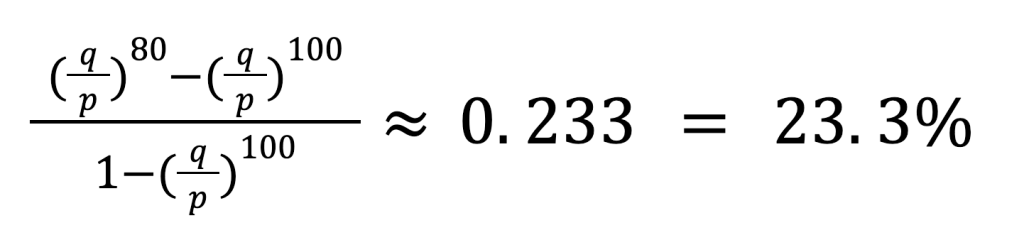
Slightly higher than in our ideal case, but it looks like Joe has decent odds of bagging that 20 pound increase. Maybe if he put more money on the table, and still aimed at the same fraction of gained wealth, things would be the same as before, right?

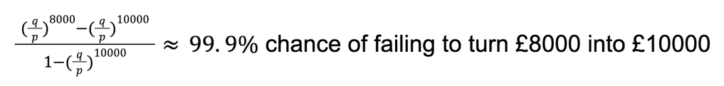
Well… that went badly pretty quickly! The general formula does not allow for nice, proportional relationships, hence the disparity in the results. Of course, anyone can tell you that it’s much harder to win two thousand pounds at a casino, as opposed to just 20, but now we have the maths to fully back this statement. Here, the quantity of potential earnings matters way more than the fraction of initial wealth related to the target wealth.

There is still a fraction that matters, though, which we have already discussed. Namely, how much you want to earn in relation to what you already have. Trying to earn £200, starting from £800, seems a bit tough, but manageable. What if Joe tries to earn £200 starting from just £1?

Financial suicide! Setting a realistic target wealth when entering a casino now depends a lot more on what you start with, rather than how much you are trying to gain. Even earning £20 from £1 can backfire 95% of the time. As for trying to multiply your fortune fast and easy? Forget about it! Turning £1 into £1000 here has a chance of epic failure of at least 99.9925%. Trying to transform £100 into £1000 has a 99% probability of sending your bank account into an early grave. In fact, even doubling your fortune from £500 seems a tough task, with an 88% chance that your account balance will bite the dust! Aiming for relatively small daily gains from your casino games is, from a probability perspective at least, much more beneficial than chasing one big jackpot.

Gambling is an insidious problem in the UK, with the NHS reporting 400,000 problem gamblers and another 2 million at risk. All gambling methods are biased against you, and if you do not bet your money responsibly by setting a reasonable maximum limit for your earnings, the maths proves that you may well end up in the position of our hypothetical gambler Joe, who ruined himself trying to reach glory. Perhaps even better is to avoid casinos entirely, but if that’s not possible then self-control is absolutely key. And, remember: maths doesn’t care about your superstitions!