Henry Jaspars – Tangled: Unravelling the Mathematics of Knots

“Incredibly detailed and entertaining in equal measure. Written with a great deal of humour and imagery helping to keep the reader engaged, whilst also ensuring the abstract ideas are made concrete and relatable for a non-specialist. I not only learned a lot about the field of knot theory, I enjoyed every moment of the journey.”

Dr Tom Crawford

Congratulations to Henry! Here is the winning essay in full.

On some level, at the very least, everyone has had some – usually frustrating – encounter with knots in their day-to-day life. Be it the fruitless attempts to disentangle a pair of intertwined shoelaces, exasperation at the inevitable encoiling of a telephone cable (which is almost obsolete, thanks to the dawn of the mobile phone), or the looping of a headphone cord with no apparent cause, the humble (yet infuriating) knot seems to have a habit of cropping up where it is least expected (and often least desired), continuing to baffle and to irritate in equal measures.

To the mathematician, on the other hand, knots are objects of profound elegance and beauty – and it is not difficult to see why. Simplicity is always of the essence for mathematicians: give-or-take, our job is less about seeing what is important to a problem, but what is not – about how much extraneous “stuff” we can remove from a problem whilst conserving the properties which matter, and in a way that keeps it behaving in a way we ought to expect. And, once you remove every unnecessary physical detail about knots, what could possibly be more elegant than a single, unbroken line coiling around itself in 3 dimensional space?

Moreover, mathematics is always (to some degree or other) about reducing the reality which we exist within and experience on a day-to-day grounding to pure abstraction – the mathematician’s home turf. From this, we can make use of this sort of analogy to better understand relationships between disparate areas which might seem unexpected at a first glance. It is small wonder that the list of knot theorists reads like a who’s-who of mathematics – from Gauss to Conway – and that the field is still full of brilliant, and fascinating personalities to this day. On a mathematical front, knots have had an illustrious and somewhat dubious history of bridging different areas of mathematics – combinatorics (the study of counting, and constructing) to topology (the study of how objects can be “like” each other in a meaningful way through continuous changes), and even into quantum computing. In short, the more we delve into mathematics, the more we realise that every road we go down will, given enough time, lead to knot theory. Paradoxically, for such a seemingly workaday, common-or-garden phenomenon, the study of knots is one of remarkable depth and ingenuity, one so simple it can be explained to anyone with a piece of string and enough tenacity, yet so complex it continues to stump mathematicians to this day.

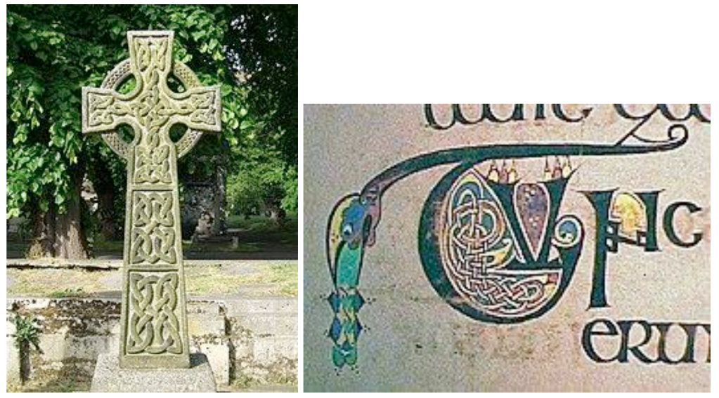
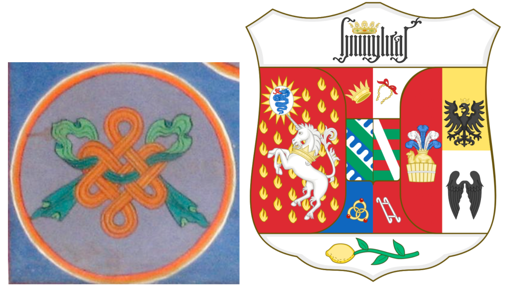
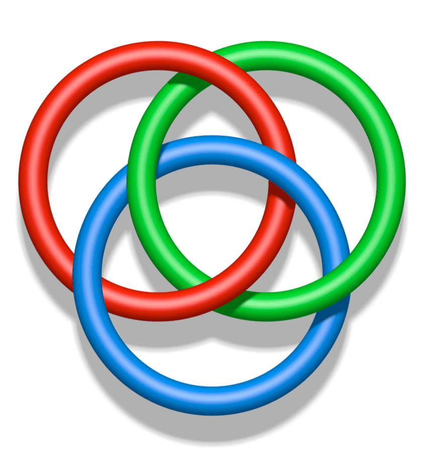
And beyond their fascination on a mathematical basis, for millennia the knot has enjoyed a universal status in various forms of spiritual imagery and as an artistic motif, too. In Celtic art, for example, the knot rears its head in illuminated manuscripts and stone carvings where it holds deep religious connotations; and meanwhile, one knot denominated the Endless Knot, having no beginning or end, is symbolic of the cycle of rebirth in Buddhism. And, in the 13th century, the pre-eminent house of Borromeo placed a fascinating knot into their family crest, now known as the Borromean links, which has the unusual property of being a Brunnian Link – namely, that they are properly linked, yet if any ring is removed, the remaining two will simply fall away!

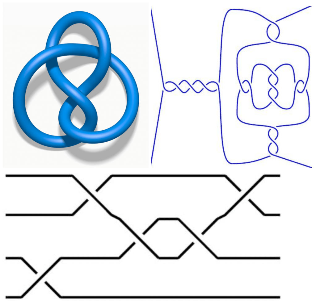
But before I proceed, it is probably helpful to have a little guide as to what exactly is a knot, and what is definitely not a knot (excuse the pun). It is a well-trodden injoke amongst mathematicians that if you have the misfortune to walk up to a topologist with your shoes tied together, they might promptly tell you that they are not knotted together, but in fact tangled, and walk off to wherever they are headed. And technically speaking, they would not be incorrect – since both laces have ends, and are not connected together in a loop, this means it qualifies as a tangle, but not a knot. And to make matters even worse, if you are speaking about interleaved strands in a loaf of bread, or in a plait, this is not a knot, or even a tangle, but a braid – which is also of interest to knot theorists, since by ‘looping’ a braid around, you can obtain the relevant knot or link (which is just a generalisation of a knot, which can have one or multiple looped pieces). And keep in mind that, if this seems somewhat contrived to have so many different words for pieces of string, please spare a thought for us poor mathematicians, who have to wrangle* with this every day.

*Contrary to popular belief, a wrangle is not a mathematical term, although I certainly wish it was.

“So, now we know a thousand-and-one things which aren’t knots, then what exactly is a knot?” I hear you cry! Well, it is usually convenient to define a knot as an embedding of the circle in 3-dimensional space – namely the image of some continuous (unbroken)embedding γ: 𝑆¹ → 𝑅³ (where 𝑆¹ denotes the circle, and 𝑅³ denotes 3 dimensional space). The most trivial embedding of all – where we just don’t knot it – is actually a knot in-and-of itself, too, called the unknot. We also usually consider two knots to be the same if there is a isotopy between them – which is just a movie which shows one knot gradually, continuously transforming from one to the other, without breaking the string, or passing it through itself – or, more formally, some continuous function

Γ: 𝑆¹ × [0,1] →𝑅³

where Γ(𝑝, 𝑡) just means the position of the point p after time t.

And in fact, this ‘movie’ trick is incredibly powerful. One famous (and surprisingly recent) result that can be shown from this is that Brunnian links (like the Borromean link I mentioned earlier) cannot be made from perfect circles – meaning that the most common diagrams of the Borromean Links are, in fact, all illusions! The proof goes as follows: assume we can create a proper Brunnian link with perfect circles. Then, construct hemispheres in 4 dimensions which have each circle as a base. It can then be seen that they don’t intersect – so just take 3-dimensional cross-sections of the whole diagram, hemispheres and all. This then gives you a movie that shows each of the links unlinking into separate circles – which is impossible, since we assumed they were linked to begin with! And it is this kind of brilliant feat of imagination which makes knot theory so fascinating to begin with.

However, although I think holograms would make this essay much more enjoyable, working in 3-dimensions can be pretty unwieldy – especially here of all places, where you are more-than-likely reading this on a screen. So instead, for convenience’s sake (and to avoid tangling ourselves up in copious amounts of string), we usually represent knots by a 2-dimensional diagram – which shows which strands of the knot pass over or under each other. Obviously there are infinitely many diagrams for the same knot, but usually we try to choose the one with the smallest number of crossing– which is known as the crossing number of a knot, or 𝑐(𝐾).

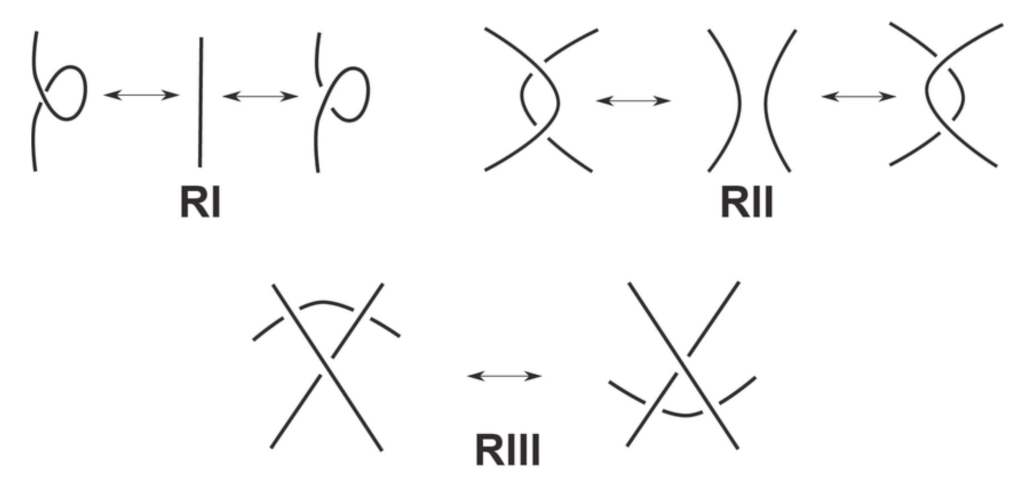
To formalise this slightly woolly notion of which knots are the same or not the same, when there are potentially infinitely many subtle variations on ways to get from one diagram to another, knot theorists have the concept of the Reidemeister moves – a collection of 3 local moves, which surprisingly are sufficient to get from any diagram to any other diagram, provided that they represent the same knot. Being an existence proof, it does not actually specify how many moves you would require to get between equivalent knots, with the current best upper bound of (239𝑐(𝐾))¹¹ – which is a 31-digit number for as few as 3 crossings – only proven as recently as 2015.

But even with these moves at our disposal, being able to show whether two knots are the same is no easy task - and in fact, checking if a knot is equivalent to the unknot (known conveniently as the unknotting problem) is widely believed, but not yet proven, to be computationally intractable - meaning that it is impossible to find an algorithm which could tell if a knot is the unknot after a time which is at most some power of the number of crossings. And even looks can be deceiving: in fact, in one famous table of over 100 knots up to 10 crossings, devised meticulously by Charles Newton Little in the late 19th century, was found to have two identical knots - now infamously known as the eponymous Perko pair - and serving as a cautionary tale for mathematics students to this day.

So if we don’t have a chance to tell if two knots are the same, how could we possibly fare better for recognising if they are different? This is where invariants come into play – an extremely versatile mathematical technique whereby we try to construct properties of an object which remain the same even when the object itself is changed. For example, in the case of isotopy as above, the number of holes an object has remains the same even if the overall shape might change*. Although this kind of technique can’t necessarily tell if things are the same (since two distinct objects might be assigned the same invariant, unless it is a perfect invariant), it can tell if two objects are not – since two equivalent objects could not possibly be mapped to the same invariant. And what makes invariants especially suited for knots is that to prove something is an invariant, we only need to show that the property doesn’t change after each possible Reidemeister move!

*Although this is hardly any use in knot theory – considering that all knots ostensibly have one hole!

One of the most intuitive knot invariants is known as 3-colourability – namely, whether it is possible to colour the arcs (connected parts) of the knot so that at every crossing, there are either 3 different colours or only 1, and exactly 3 colours are used overall. This can be seen to be a knot invariant: we can always tweak our colouring to ensure that the colouring condition still holds. So, since the unknot is not 3-colourable (since fewer than 3 colours will be used), and since the trefoil is, not all knots are equivalent to the unknot!*

*Despite the fact that this might seem really obvious at first glance, bear in mind that proving it beyond all reasonable doubt is actually quite hard, as we’ve seen here – although a proof that ‘a knot is actually knotted’ probably provides little solace to anyone who is actually trying to undo one. Oh well.

And, in fact, this method can be generalised to a more powerful technique known as Fox n-colourings. Here, instead of assigning a colour to each arc, we assign a number modulo* n, such that at every crossing, the following relation holds: a + b ≡ 2c (mod n).

*If you aren’t familiar with modular arithmetic, just think of them as considering two numbers to be the same modulo n (written as x ≡ y (mod n)) if they share the same remainder when dividing by n – so, for example, 12 ≡ 33 (mod 7), both leaving remainder 5 when dividing by 7.

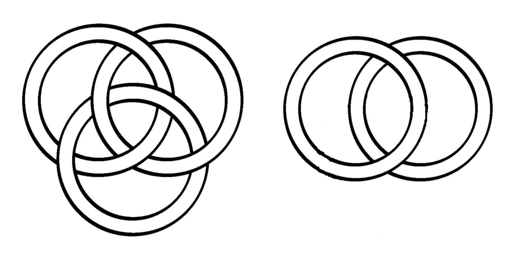
The invariant, in this case, is just the number of distinct solutions where the value of each arc is taken to be between 0 and n – 1. And, in fact, we can see that this is incredibly powerful: whilst we cannot distinguish the Borromean links from the unlink (just 3 unlinked circles) with 3-colouring (which is equivalent to the case n = 3), we can do this with Fox colourings – choosing n = 5, we end up 125 colourings for the unlink (5 choices for each circle), and only 5 for the Borromean links – and hence showing that they are, in fact, linked after all.

However, a single number is usually inadequate to distinguish between knots which might not yield to the above techniques. What we need instead is a polynomial – an expression which is a sum of the powers of some variable or variables (so for example, 1 + 2 · 𝑡⁻¹ + 𝑥³ · 𝑡 is a polynomial in 𝑥 and 𝑡). The earliest of these is by far the Alexander polynomial – named after the late 19th-century American topologist James Waddell Alexander II, who is also well known for his infamous Alexander horned sphere, a notorious pathological object (namely, one which haunts the nightmares of mathematicians). His polynomial, at any rate, is much more pleasant, and can be concocted with the following recipe:

1. For each crossing, labelled as above, write down the following equation: c + tb – tc + a = 0
2. For each arc of the diagram, create a matrix (2-dimensional array) of the coefficients from each equation in 1) – with a row for each crossing, and a column for each arc;
3. Choose your least favourite row and column, and delete them;
4. Then just calculate the determinant* of the matrix!

*A determinant is a single value constructed from a square (with as many rows and columns) matrix. For a 2 x 2 matrix, this is the area of the parallelogram formed by the vectors of each column.

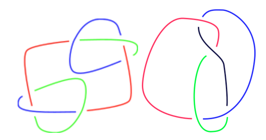
Remarkably, this does not depend upon choice of diagram (as long as there are no closed loops). This polynomial, denoted ∆_𝐾(𝑡), has nice properties: firstly, that it is symmetric – namely, that ∆_𝐾(𝑡) = ∆_𝐾(1/𝑡) – the useful property that it behaves nicely with knot sums – if 𝐾 # 𝐿 denotes the sum of two knots, then ∆_𝐿#𝐾(t) = ∆_𝐿(𝑡) · ∆_𝐾(𝑡) where 𝐾 # 𝐿 is constructed by cutting a small ‘gap’ in each knot, and joining them together as below:

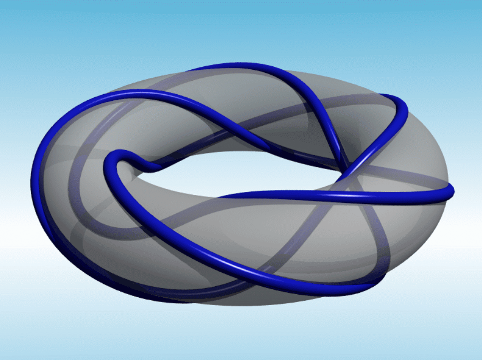
Curiously, we can define prime knots naturally from this definition: namely, all knots K such that, if we have 𝐾 ~ 𝐿 # 𝐿’ for knots 𝐿 and 𝐿’, then one of 𝐿 or 𝐿’ are equivalent to the unknot (compare this with a number n being prime if, whenever 𝑛 = 𝑎 × 𝑏, then one of 𝑎 or 𝑏 must equal 1). And in fact, from the Alexander polynomial, we can see that there are infinitely many prime knots: a specific family of knots known as torus knots, which can be formed by wrapping a piece of string around a torus, can be seen to have Alexander polynomials which don’t factorise, and hence have to be prime knots!

On a historical aside, though, for a lot of the 20th century, interest in knot theory had more or less evaporated. To understand why, however, it is vital to know exactly why knot theory was studied to begin with. The kind of knot theory we would recognise today was invented by Lord Kelvin – of ‘degrees Kelvin’ fame – who thought at the time that the distinct properties of each atom came from a knotted hole in what was called the luminiferous aether – the medium through which light was thought to travel. And as much as this might seem ridiculous today, it had an immense amount of credibility at the time, and leading scientists of the day – including J. J. Thomson (who would go on to discover the electron) and James Clerk Maxwell (who is celebrated for his unification of electricity and magnetism) – and sparked a flurry of research into knot theory, spearheaded by Peter Guthrie Tait, who published the first tables of knots. Of course, in hindsight they were very far from the truth – as was proven by the Michelson-Morley experiment, acrimoniously dubbed “the most famous failed experiment of all time” – and resulted in a mass abandonment of the knot theory gold rush. In defence, it could also be argued that this false hypothesis was no cul-de-sac – for, if no-one had pursued that avenue for thought, it is likely that knot theory as we know it today might never have existed in the first place.

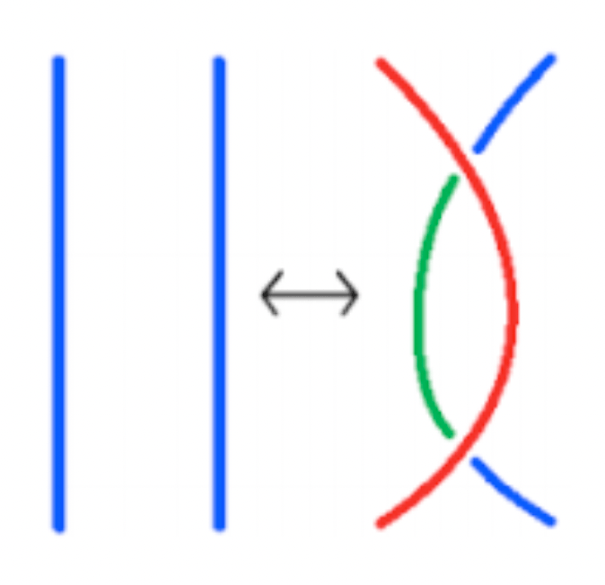
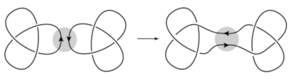
In any case, this stasis continued until the pioneering work of Vaughan Jones, a truly brilliant mathematician (who, ironically, had a background in von Neumann algebras – a field closely related to quantum physics) whose discoveries earned him the 1990 Field’s medal – the highest accolade in mathematics, which, as a true New Zealander, he received wearing an All Blacks rugby jersey. The origins of his most lauded discovery, the Jones knot polynomial, are still a mystery amongst mathematicians. Legend has it that the result simply appeared one day on the department’s communal blackboard with little fanfare at its arrival – despite rejuvenating the entire field of knot theory. The result is a simple, recursive formula: if we produce links 𝐿₊, 𝐿₋ and 𝐿₀ by altering a single crossing as shown, then the skein relation says that the Jones polynomial should follow:

(𝑡^1/2 − 𝑡^−1/2) 𝑉(𝐿₀) = 𝑡⁻¹ · 𝑉(𝐿₊) − 𝑡 · 𝑉(𝐿₋)

And as much as this might seem less intuitive than the Alexander polynomial – even to see that this doesn’t depend upon how we apply the relation – the resulting polynomial has many more remarkable properties. For example, the Jones polynomial can sometimes distinguish between a knot and its mirror image, provided that they are distinct (known as chirality), which is never true for Alexander polynomials.

Moreover, if a knot is alternating (i.e, goes over-under-over-under… in reduced form, i.e, with no ‘loops’), then the coefficients of the Jones polynomial will also be alternating (i.e, if you write 𝑉(𝐿) = 𝑎₀𝑡^𝑑₀ + 𝑎₁𝑡^𝑑₁ + 𝑎₂𝑡^𝑑₂ + … for 𝑑₀ < 𝑑₁ < 𝑑₂ … and 𝑎_k ≠0 then 𝑎_k will have changing signs). In fact, this result settled the century-old conjecture from P. G. Tait that reduced diagrams of alternating links cannot be drawn with fewer crossings – testament to the immense power of Jones’ discovery.

Jones’ result was also lauded for bringing back attention to low-dimensional topology – and the connection between the two subjects is not immediately obvious. Earlier than Jones, William Thurston (who also won the Fields Medal) had found a link between 3-dimensional manifolds (a topological object which looks like 3-dimensional space from every point) and knot theory – giving rise to a fascinating invariant known as hyperbolic volume (which is sadly beyond the scope of this essay).

But even earlier than that, seminal topologist Herbert Seifert had discovered the eponymous Seifert surfaces – a subject of fervent research to this day, and which look as if someone had made a knot out of wire and dipped it into bubble mixture. A Seifert surface is simply an oriented (i.e, with 2 sides, unlike a Mobius strip, which is unoriented) surface whose boundary is the knot itself. Properties of this manifold actually yielded methods to approach the unknotting problem which was mentioned earlier – which on the front of it is completely unexpected. This makes more sense when we see that this gives rise to a useful knot invariant known as the knot genus, denoted 𝑔(𝐾) – which is just the number of holes that the resulting surface has (and which is miraculously invariant on the choice of surface, and how we draw the knot). It turns out that the only knot with genus 0 is the unknot – and furthermore, that

𝑔(𝐾#𝐿) = 𝑔(𝐾) + 𝑔(𝐿)

– i.e, that the number of holes for knots K and L ‘adds up’ when we take their knot sum. This shows that, in fact, inverse knots cannot exist – since if we did have K, L such that K # L is the unknot, then both K and L have to be the unknot – since otherwise, 𝑔(𝐾) + 𝑔(𝐿) ≥ 1 (since they can’t both be the unknot), but 𝑔(𝑢𝑛𝑘𝑛𝑜𝑡) = 0 – which is impossible! Which all begs the question – is it to be, or knot to be?