
Gavin Jared Bala
In a wine cellar, a mine, or any other deep underground space, we notice an interesting phenomenon. Despite the lack of any visible heating, the temperature seems surprisingly stable, constant, and comfortable. Why?
The answer comes from the heat equation, a partial differential equation that mathematically models the conduction of heat!
At the scales we typically build wine cellars, the Earth might as well be considered infinite. It can be well-approximated as a flat plane and everything below it. In fact, we don’t have to worry about our exact location on Earth’s surface: the temperature doesn’t change much moving a few metres on the surface. So we only need to consider our depth.

Let’s set up our variables.
Define x as depth and t as time, and let T(x,t) be the temperature of the soil at depth x and time t. Note that this is a function of two variables, not of just one.
Further, let q(x,t) be the heat flux (the flow of heat energy) in the positive x direction (downward) at depth x and time t. (So -q(x,t) would be the heat flux in the negative x direction at the same point.)
Finally, let ρ be the density of the soil (in kilograms per cubic metre) and c be its specific heat capacity: the amount of heat required to raise the temperature of one kilogram of the soil by one degree Celsius. Multiplying it by the density gives the product ρc: this is the volumetric heat capacity, which is the amount of heat required to raise the temperature of one cubic metre of the soil by one degree Celsius. So the product ρcT(x,t) measures the heat energy at depth x and time t.
To find the heat energy contained in the soil from depth a to a+h, we have to integrate the product ρcT(x,t) across this interval, giving

(Note that we are integrating over depth, not over time!) The net heat flux into this interval equals q(a,t) – q(a+h,t) (as we want the downward heat flux at x = a and the upward heat flux at x = a+h).
Now, the law of conservation of energy tells us that the rate of change of this internal energy must equal the net heat flux. The rate of change is, as usual, represented by a derivative. So we formalise this as:
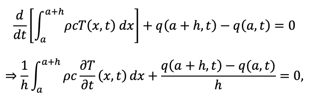
We moved the derivative past the integral sign (the Leibniz integral rule). Although some rigorous justification is required to do this, the intuition is clear: the integral is being taken over limits that do not vary with t, so the differentiation and integration can be swapped in order.
The funny ∂ indicates that this is a partial derivative. T is a function of two variables, but we’re only taking the derivative with respect to one of them. We pretend the other is a constant. If we plot it as a 3D graph above the x,t-plane, we can think of this procedure as taking a cross-section of the graph across a line of constant x. This leaves a 2D curve that’s a function in t only, and then we can take the derivative as normal.
Finally, we let h approach zero to examine the local situation. The fraction clearly becomes a derivative, taken this time in the variable x (as that’s the one that varies). The first integral is divided by the length it ranges over, and can be thought of as an average value over its interval. Hopefully you will agree that as the interval shrinks to a point, the average must go to the single value at that point.
Thus the equation becomes
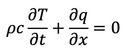
We don’t need to specify a, because it was arbitrary: the same logic would have held at any depth.
Now, this still has too many variables: we don’t know how temperature and heat flux relate to each other. This is where we need some more physics.
Fourier’s law of heat conduction, named after French mathematician Joseph Fourier (1768–1830), states that heat flux is proportional to the negative gradient of the temperature:
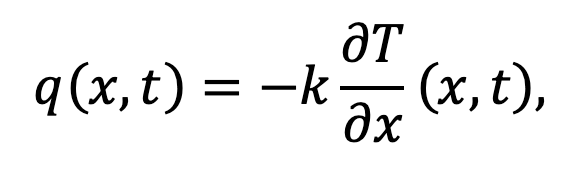
where k is thermal conductivity. As I’m sure most of us are aware, heat flows from hot to cold and flows faster in a more conducting material, both of which are represented in the above equation.
Substituting this in gives the final form of the heat equation:

where κ is a new quantity, thermal diffusivity.
We can now tackle the wine cellar problem: how deep should we build a wine cellar to counteract surface temperature fluctuations?
The temperature variation across the year is primarily controlled by the seasons. We thus expect a periodic solution for the heat equation, as the seasonal cycle repeats: it can be approximated by sine-wave temperature variations. As the seasons don’t depend on depth, the variables depth and time should appear separately.
The simplest periodic functions are the trigonometric functions, sine and cosine. So we’ll seek a solution that reduces to a sine wave on the surface (zero depth). But sines and cosines turn into each other when differentiated, so we’ll employ a useful trick to keep things simpler!
By Euler’s formula, eix = cos x + i sin x. This turns trigonometry into exponential functions, which are easier to differentiate. So we want a complex-valued solution of the heat equation of the form
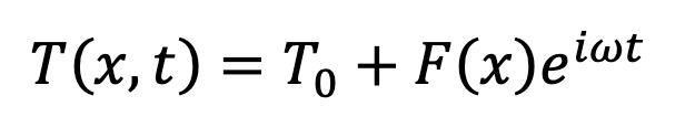
Here ω represents the frequency of the seasonal temperature oscillations, which will be 2π/1 year = 2.0 x 10⁻⁷ s-1. T0 is a constant average for the temperature to oscillate around. As a constant, it vanishes in the differentiation.
Now, you may be asking when is such a candidate solution compatible with the heat equation? Well, this solution is separable apart from the additive constant. This means that the term F(x)eiωt is the product of a function of x with a function of t. Therefore, it is easy to compute the partial derivatives (remember that to do so, we pretend that the other variable is a constant):
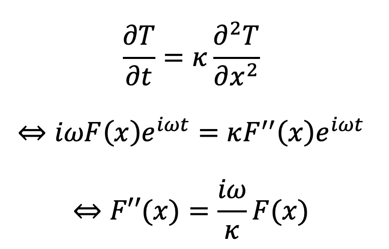
This is an ordinary differential equation for F(x)!
How do we solve it? Well, what function is its own derivative? The exponential, ex. How do we make the derivative scaled by a factor a? Well, by the chain rule, we need eax, whose derivative is aeax. But we have a second derivative, which will be a2eax. So, to solve this, we need to find the square roots of our factor iω/κ.
This reduces to finding the square roots of i, as ω/κ is real. In terms of what it does to the complex plane, multiplying by i is just a rotation by 90° (which equals 450°) anticlockwise: in particular, it sends 1 to i on the complex plane. A square root should do half of that, i.e. rotate by 45° or 225° anticlockwise.

So, it should send 1 to somewhere on a 45° angle from the real axis, i.e. where the real and imaginary part are equal; but it should stay at distance 1 from the origin. Clearly, this must be

So, the square roots of iω/κ are

Therefore, the general solution is a linear combination of the two possible exponentials:
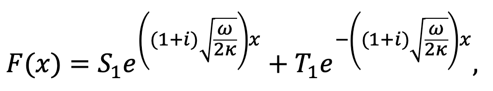
where S1 and T1 are arbitrary constants. (We can add the two candidate solutions because differentiation is linear.)
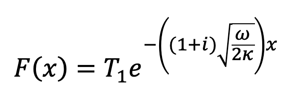
However, the first term contains a positive exponential factor, which is physically impossible: the temperature fluctuations do not get arbitrarily large with increasing depth, as they cannot pass absolute zero. Therefore, S1 must in fact be zero, and we just have one constant:
Decoupling real and imaginary parts by Euler’s formula again, we get (exp(x) = ex):
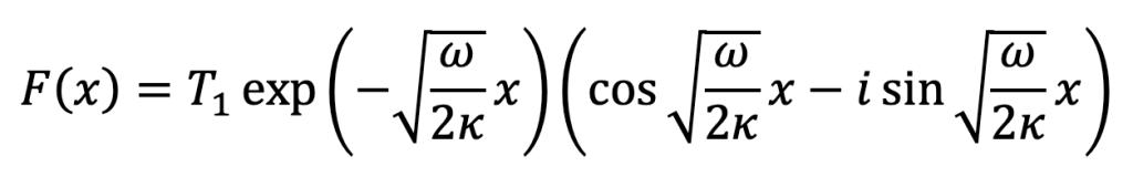
Differentiation is linear, so the real and imaginary parts of a solution to a differential equation also satisfy the same differential equation. This finally gives us a solution of the form:
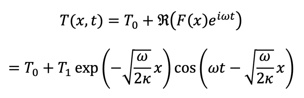
(The fancy R refers to taking just the real part.)
At ground level x = 0, this reduces to the expected sinusoidal temperature dependence on the seasons:
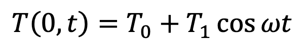
The constants are thus explained as:
- T0 = (Tmax + Tmin)/2 (the average temperature)
- T1 = (Tmax – Tmin)/2 (half the range of temperature variations)
The rate of change of temperature with depth is:

By our choice of the negative exponential, ∂T/∂x vanishes as x approaches infinity.
To counteract the seasonal cycle on the surface, we choose depth to bring us maximally out of phase with it, i.e. pick such that (ω/2κ)1/2x is an odd multiple of π. For Earth’s soil, κ = 10-6 m2 s-1, and plugging in the numbers gives us a minimal ideal depth of 10 m for our wine cellar.
Because of the exponential damping of the oscillations, we find ourselves at a near-constant average temperature T0 quite quickly!
So, there you have it. The next time you find yourself digging out a cellar to store your wine, remember maths has the answer.

[…] the heat equation is not only important for wine cellars (see previous article). We’ll look at a much larger-scale and very faraway situation where it plays a key […]
LikeLike