
Gavin Jared Bala
One of the two basic operations of calculus is differentiation.
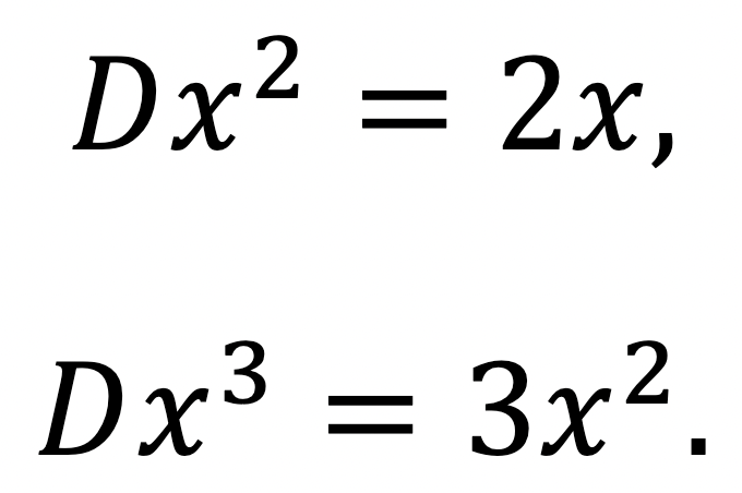
Differentiation finds the slope of a function f(x) at one point. This produces a new function known as the derivative:
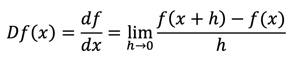
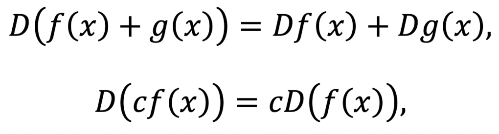
The notations df/dx and f'(x) for the derivative are common, but here we want to emphasise that the derivative is really an operator. Unlike a function, which takes a number and returns another number, an operator takes a function and returns another function. So we will write the differentiation operator as D, which when applied to the function f(x) returns the derivative Df(x) = df/dx.
Calculus can be seen to have a special connection with the infinitely small, as differentiation is a limiting procedure as something goes to zero. Travelling on the graph from x to x + h, we rise a distance of f(x + h) – f(x) and run over a distance of h. This gets us the average slope over this distance, and we hone in closer and closer to the instantaneous slope at x as h becomes smaller and smaller.
But there is an analogue called finite calculus!
Consider what happens before we pass to the infinite world: we only can examine our function at individual steps. Perhaps something coarse like 1, 2, 3, 4, …; or perhaps something finer like 1, 1.05, 1.1, 1.15, …; but the step size is really not that important (it can be scaled), so we will assume that it is always 1.
In this case, we have something that might look familiar: it is a sequence. Sequences can be thought of as a type of function where we only allow integer inputs.
For example, the sequence corresponding to f(n) = n is just:
1, 2, 3, 4, 5, 6, 7, 8, 9, 10, 11, 12…
Slightly less dull is the sequence corresponding to f(n) = n2, which gives the square numbers:
1, 4, 9, 16, 25, 36, 49, 64, 81, 100, 121, 144…
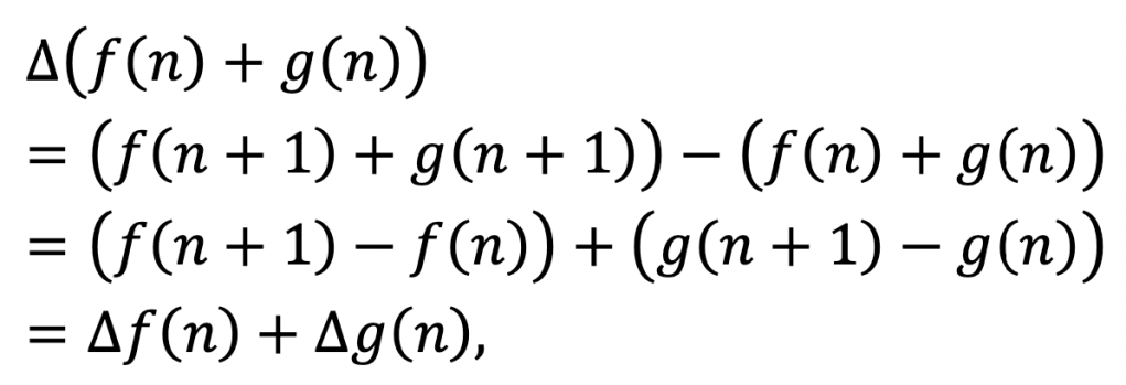
So what is the appropriate analogy to the derivative? It is the difference between successive terms! We write △ for the difference operator:
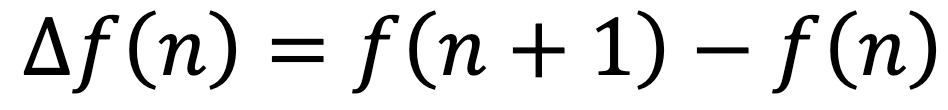
Since 1 is our smallest step size; we are working discretely and can go no finer. So this really already is the instantaneous change at a point!
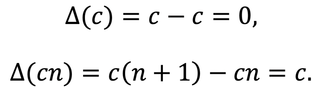
Now, what functions do we first learn to differentiate? Constants and linear functions, for they have very simple derivatives. If is a constant, then:
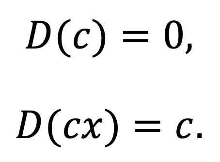
Just the same is true, as expected, for differences.
We can also easily see that differentiation is linear:
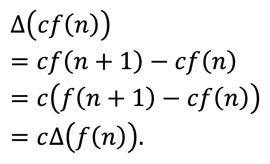
and so is the difference:
and
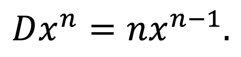
The next functions we typically learn to differentiate are perfect powers, by the power rule:
For some specific cases,
This works for any complex power n when understood correctly, but at the moment we’ll just think about integers.
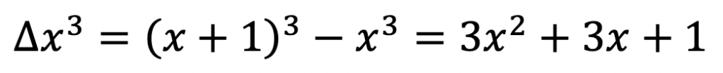
How does that work for differences? Well, not quite as immediately well. Let’s work out

which is almost right, but has an annoying shift.
But we’ve already seen that taking the difference is linear, and we know that △x = 1. So, we have:
And for the next power:
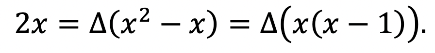
is no good, but we have
which returned our substitute for x2 (since we saw above that differentiating x(x – 1) will return 2x, the ‘usual’ derivative of x2).
This suggests that just as the normal definition of powers worked nicely with derivatives, there will be a new kind of power that works nicely with differences, which takes into account the finite step size. This is descriptively called the falling factorial (or falling power), and given a notation that suggests its analogy to powers:

Note that this product has n factors. The underline (Donald Knuth’s notation) emphasises that the factors fall.
The ordinary factorial is a special case: x! = x_x. And just as with powers, x_1 = x.
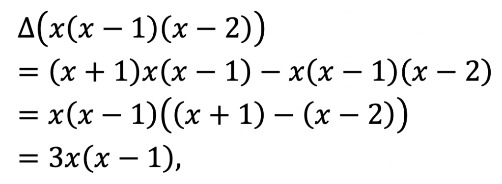
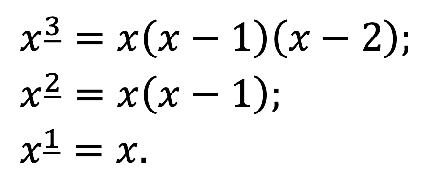
And we can see, just like we did for x_3 = x(x – 1)(x – 2) above, that this really does work in general:
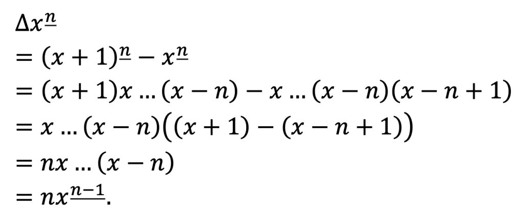
This is the power rule for differences.
Just as we can differentiate general polynomials term-wise by linearity, so we can do the same for differences. But to do it more easily, we should express them in terms of falling factorials rather than powers.
For example, we could have calculated △x3 by expressing
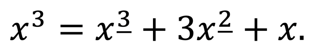
This would allow us to take the difference term-wise:
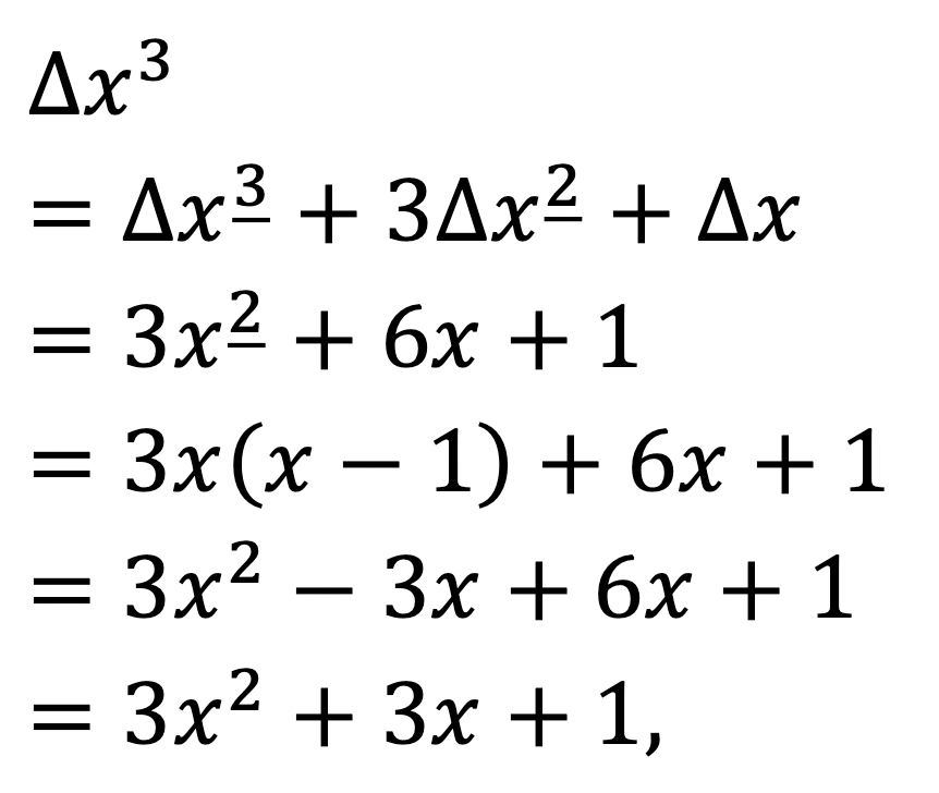
agreeing perfectly with our earlier answer!
In general, we can always get this kind of expression by comparing coefficients. The coefficients we get from expressing xn in falling factorials, or from expressing x_n in normal powers, are actually a famous set of combinatorial sequences called the Stirling numbers.
Now, the definition of power extends perfectly to any integer power, but how do we do this for falling factorials?
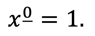
Just as x0 seems to be an empty product of no terms, the same holds true for x_0; so the natural definition for that is 1.
This is justified by noticing the pattern:
To get from x_3 to x_2, we divide by (x – 2); to get from x_2 to x_1, we divide by (x – 1). It therefore stands to reason that to get from x_1 to x_0 we should divide by x, yielding
Indeed, there is no reason we should stop there. To pass from x_0 to x_-1, we should presumably divide by (x + 1), and then keep going:
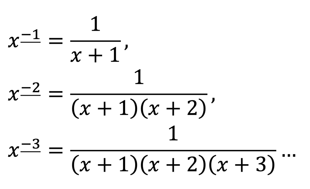
And so on!
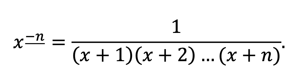
Generally,
We’ll now verify that the power rule really does apply even to those negative falling factorials:
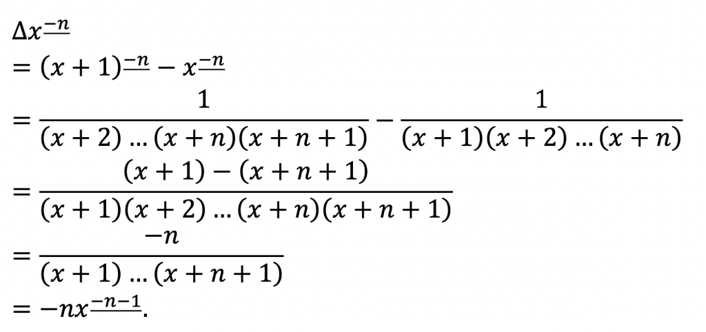
Yes, it works!
We can in fact define x_n even when n is not an integer, but it gets complicated: it involves the gamma function, which is a continuous version of the factorial. So we’ll stick to integer cases.
Trying to generalise the power rule has borne a great deal of fruit. So it’s now natural to ask the question: can we learn more about finite calculus by trying to generalise the other rules of differentiation? Say, the product rule, the quotient rule, or the chain rule?
Alas, the chain rule isn’t particularly amenable to working with finite calculus: substitution gets a little bit dicey in the discrete world.
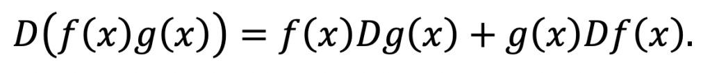
But let’s try the product rule. First, recall what it looks like in the normal infinite calculus:
Now, let’s try to find the difference of a product!
By definition,

Now we employ a very useful trick. We want to vary one of the function inputs at a time, but currently, both are being varied. So we will add and subtract an intermediate term:
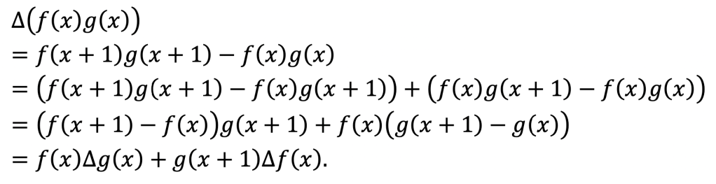
And that’s it!
It looks almost like the product rule of infinite calculus. The only difference is just like what happened for powers versus falling factorials: there is a shift of the input at one point, because we have a discrete step size now. (In the infinite calculus, we would have an h here in the derivation that goes off to zero and vanishes.)
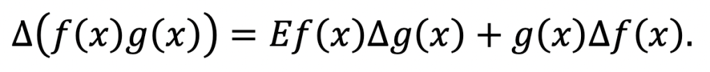
To save ourselves some writing, we can invoke the shift operator E:
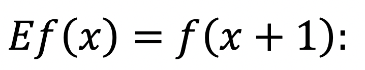
it shifts the input over by one. Thus we can write

The symmetry break is only apparent. For we could have added and subtracted f(x + 1)g(x) instead, and then we would have obtained the equivalent expression
The analogous quotient rule is easily derived after considering △[1/g(x)].
Now, I need to make a confession. So far, we have only covered one half of calculus… For not only is there differentiation, but also its inverse operation, integration. The indefinite integral or antiderivative of a function is something that can be differentiated to give back the original function. And this is exactly what we will be investigating in the second part of this article…
References
Graham, R. L.; Knuth, D. E.; Patashnik, O. (1994). Concrete Mathematics. (2nd ed., pp. 47–56). Addison-Wesley.
Kelley, W. G.; Peterson, A. C. (1991). Difference Equations: An Introduction with Applications. (pp. 15–36, 70–78). Academic Press.

[…] back! In part I we introduced the notion of finite calculus with a discussion of differentiation. We will now […]
LikeLike
A very interesting post introducing a new topic for me!
With regard to the chain rule, it is interesting to look at the permutation invariant form:
Delta(fg)=0.5[(g+Eg)(Delta(f)) + (f+Ef)(Delta(g)]
(f+Ef)/2 is of course just the average of f(x) and f(x+1) and so can informally be thought of as f(x+0.5): here we see a link to the famous midpoint rule for computing finite distances!
LikeLike
[…] for Divisibility of ANY Number The Finite Calculus: Part I Differentiation 5 Types of […]
LikeLike