Gavin Jared Bala

Welcome back! In part I we introduced the notion of finite calculus with a discussion of differentiation. We will now continue with the second half of calculus: integration – often seen as the inverse operation to taking a derivative. The indefinite integral or antiderivative of a function is something that can be differentiated to give back the original function.

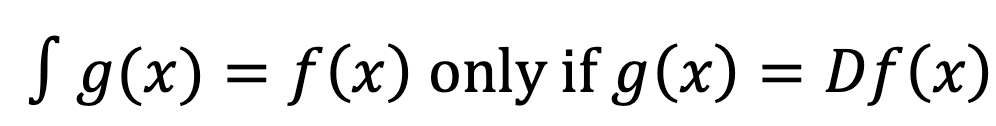
Although we really should not have used the definite article there: for a constant differentiates to zero, and hence if g(x) = Df(x), then also g(x) = D(f(x) + c) for any constant c. Therefore, we had better make it indefinite up to a constant:

That’s better!

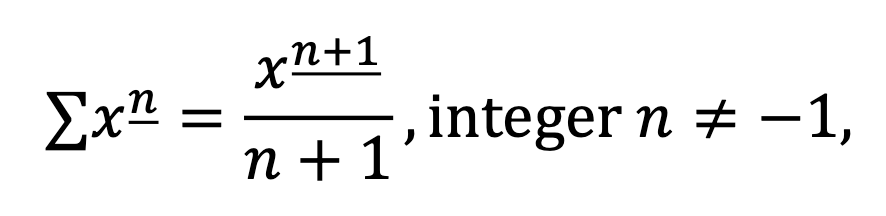
Analogously, in finite calculus, the difference operator has an inverse operation, giving the indefinite sum:

(Just as Latin D became Greek Δ, thus Latin ∫ became Greek Σ!)

In this case, c can be any function such that c(x + 1) = c(x). We might have c constant, or we might have another periodic function like c(x) = c cos(2πx).

And there is also a definite integral: it is defined as

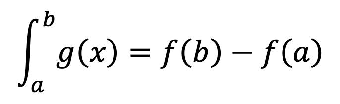
where f(x) is an indefinite integral of g(x).

Completely analogously, there is also a definite sum, which is:

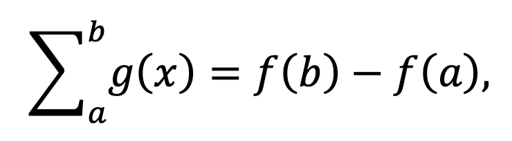
where f(x) is an indefinite sum of g(x).

We can justify this name. For f(b) – f(a) is a telescoped sum:

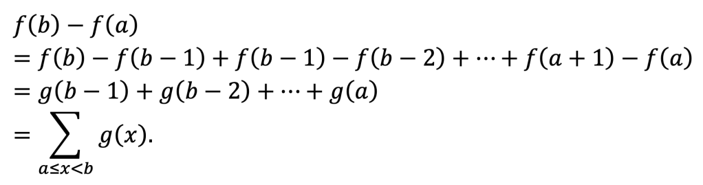
Unfortunately this clashes a little with the usual notation (in which Σ_a^b g(x) means g(b) + g(b – 1) + … + g(a) = Σ_a<=x<=b g(x), but we will keep it this way to reinforce the similarity with the definite integral.

Therefore, we can see that the finite calculus can be used to calculate sums!

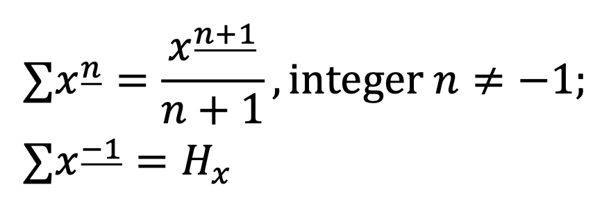
By reversing the power rule calculated in part I, we can deduce that

and therefore we can derive formulae for the sums of n^th powers by expressing them in terms of falling factorials.

For example, we know that x² = x^_2 + x^_1, and therefore we deduce that

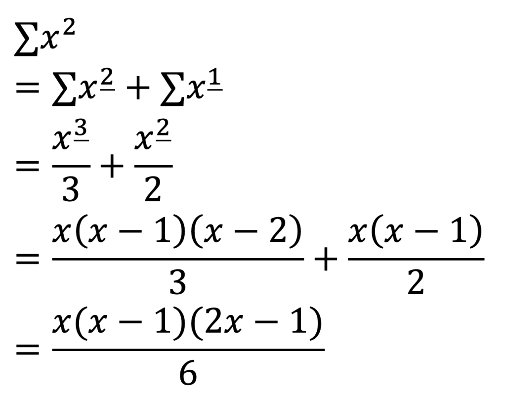
To get the constant, we need some initial conditions, just as for the indefinite integral. This is easy to get from the trivial terms: the sum of no squares is 0, and the sum of the one square 1 is just 1. So we get

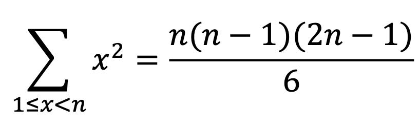
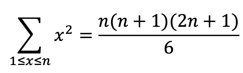
This is more normally written including both ends:

Similar expressions may be found for sums of n^th powers, called Faulhaber’s formulae.

We also recall that in the power rule for integration, there was a logarithmic special case:

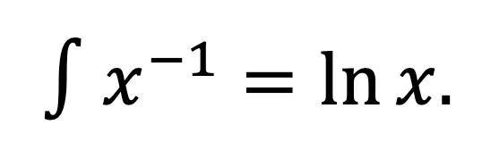
So, there is also one special case among the falling factorials that cannot be written in terms of functions we already know: Σx^_-1. It must be a sequence whose differences form the sequence 1, 1/2, 1/3, 1/4, 1/5, …

One such sequence is the so-called harmonic numbers:

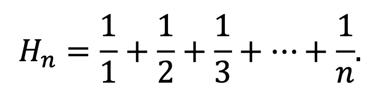
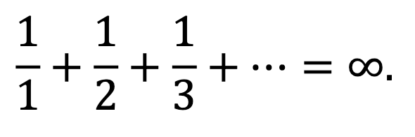
They are named thus because they are the partial sums of the harmonic series

Thus we can fully complete the summation power rule:

In fact, the harmonic numbers are deeply related to the logarithm, further cementing the analogy: the error between ln(x) and its discrete analogue H_x approaches the Euler-Mascheroni constant γ = 0.5772… as x gets large.

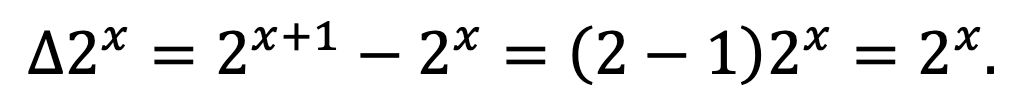
Just as there is a logarithm analogue, there is also an exponential analogue: a function that is its own difference. In fact, it is also an exponential, although this time the base is even more familiar than e. For it can clearly be seen that

The situation for other exponentials is almost as simple: just as for differentiation, a factor is picked up.

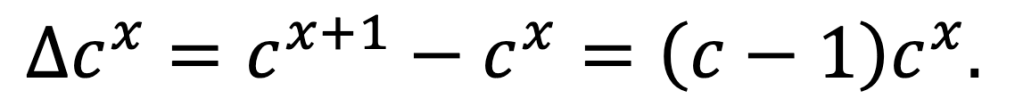
In fact, this is even nicer with the shift operator (see part I), as it then becomes Ec^x = c^x+1 = cc^x with complete analogy to differentiating exponentials: De^cx = ce^cx.

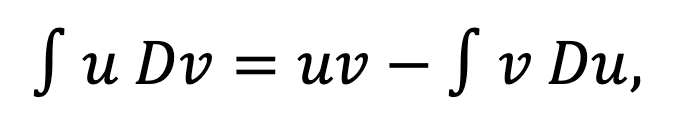
And just as we can reverse the product rule of differentiation to give integration by parts:

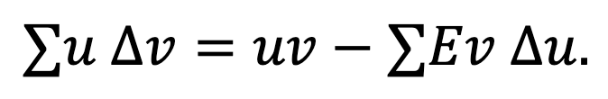
so reversing the product rule of differences gives summation by parts:

We will demonstrate this via some examples, emphasising each time the analogy between summation and integration:

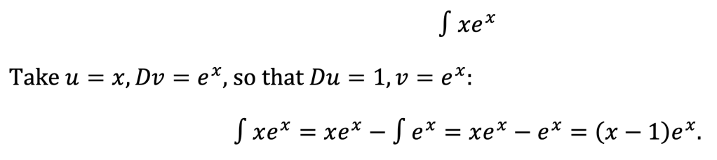
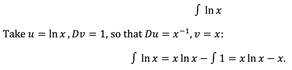
Integration, Example 1:

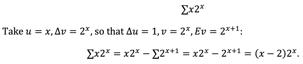
Summation, Example 1:

Integration, Example 2:

Summation, Example 2:

We will conclude with one last analogy, this time between differential equations and difference equations.

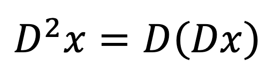
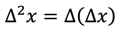
Recall that in calculus, the second derivative is the derivative of the derivative:

Analogously, we can define the second difference as the difference of the difference:

Third and higher derivatives and differences continue in exactly the same way.

A differential equation is an equation for a function f(x) in terms of its derivatives. A major class of differential equations are those with constant coefficients.

Suppose we have a differential equation with constant coefficients

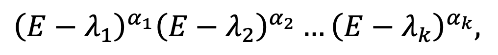
The differential operator in brackets, being a polynomial in D, must factorise as

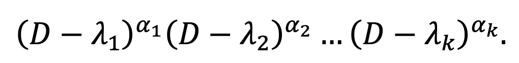
(The roots can be complex.) So, we simply need to solve the equation (D – λ)^α f = 0. The simplest case is α = 1, in which case we have just e^λx. In general, the solutions will be e^λx, xe^λx, … , x^α-1e^λx.

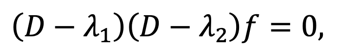
So, it turns out that the general solution is a linear combination of these for every α and every λ. In the most common second-order case, we have

which is solved by

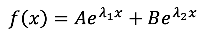
if λ₁ ≠ λ₂, or

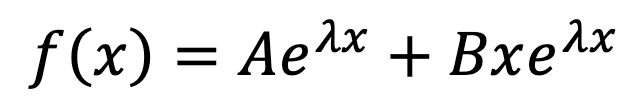
if λ₁ = λ₂ = λ.

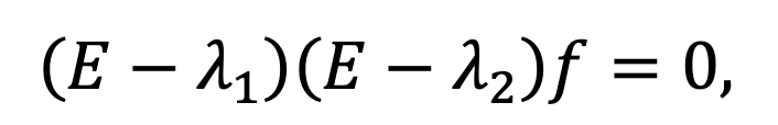
Well, the same thing happens when solving a linear recurrence. A recurrence of the form

can be rewritten using the shift operator as

This operator factorises as

and the solutions of the equation (E – λ)^α f = 0 are just λ^x, xλ^x, … , x^α-1λ^x. In the second-order case, we have

which is solved by

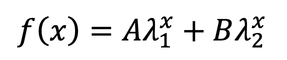
if λ₁ ≠ λ₂, or

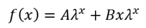
if λ₁ = λ₂ = λ. Notice the complete analogy! (In both cases, when complex numbers appear as roots, it may be better to change from exponential to trigonometric form.)

We will finally use our new tools to derive Binet’s formula for the Fibonacci numbers. The Fibonacci numbers are famously given by the recurrence relation

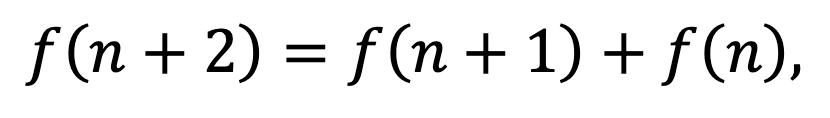
in which every term is the sum of the previous two.

This can be rewritten in terms of shift operators as

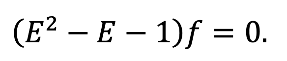
By applying the quadratic formula, we can see that x² – x – 1 has two roots:

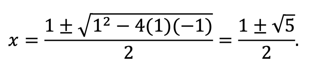
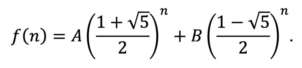
The positive root (with the + sign) is the golden ratio, often symbolised ϕ or τ. So, by the above, we have:

Finally, we need to determine the constants. In the standard Fibonacci sequence, we have f(0) = 0, f(1) = 1. Therefore we have two simultaneous equations to solve, one coming from each initial condition:

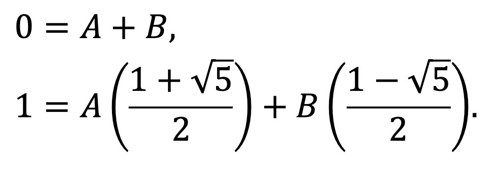
The first equation tells us that B = -A, so the second becomes 1 = A5^1/2. Thus A = 1/5^1/2 and so

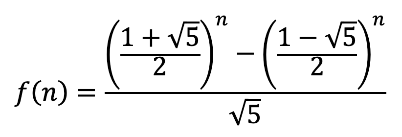
It is certainly an astonishing sight to see how this formula, in spite of all the appearances of 5^1/2, always gives integer values for integer inputs!

So, the next time you see a difficult sum or recurrence, astonish your friends with the power of finite calculus!

---

References

Graham, R. L.; Knuth, D. E.; Patashnik, O. (1994). Concrete Mathematics. (2nd ed., pp. 47–56). Addison-Wesley.

Kelley, W. G.; Peterson, A. C. (1991). Difference Equations: An Introduction with Applications. (pp. 15–36, 70–78). Academic Press.