Ioana Bouros

Why do children look so similar to their parents? For example, why do they tend to have the same colour hair or eyes? This type of behaviour is what we call genetic inheritance and such questions have perplexed scientists and thinkers for many centuries. Even today, we do not have complete knowledge of how traits are shared from one generation to the next, but in the last century and a half extensive discoveries have been made, and the problem continues to be worked on. Remarkably, it’s a piece of clever mathematics that led to the initial breakthrough that started it all…

So, who is responsible for this new era of enlightenment? The father of modern genetics if you will? Any biologist worth their salt will tell you that there is no one answer. In fact, for quite a while two theories regarding the process of inheritance were in circulation in the academic world until their final reconciliation (thanks to Fisher, Haldane and Wright) at the beginning of the 20th century. These two theories are the evolutionary theory brought forth by Charles Darwin and the theory of allelic inheritance of Gregor Mendel. The former believes that the wide variety of traits we see in individuals is due to the accumulation of changes that occur over long periods of time in the history of a species, the so-called mutations; while the latter states that characteristics are inherited from our ancestors in blocks (called genes, with each version that manifests differently called an allele). Of course, neither completely explains what exactly happens; the reality is much more complicated.

In this article, we will concentrate on the second of the two theories stated above. Why? Because, apart from being the first to emerge – the “spark” that started it all – it came about in the most, let’s say, unconventional of ways.

Gregor Mendel was neither a biologist, nor a naturalist, nor a mathematician – in fact he wasn’t even a proper scientist in any sense of the word. He was a monk, and while in the Middle Ages it may have been true that most of the thinkers were members of the clergy, this was certainly not true by the 19th century. Now, you may be wondering, how does a monk end up dealing with genetics? 

He was not looking for answers into human nature that day, but rather spending his time gardening: he had multiple varieties of pea plants, which he was aiming to crossbreed. They were either green (G) or yellow (Y) in colour, with a smooth (S) or wrinkled bean. He observed some rather interesting things when crossing such disparaging varieties. By crossbreeding one plant yielding green and smooth beans and the other yielding yellow and wrinkled beans, he obtained pea beans of all possible combinations: yellow and smooth, green and smooth, yellow and wrinkled and green and wrinkled. 

Out of a total of 556 beans produced by the grafted plant, the distribution of the types of resulting beans was as follows:

Based on these numbers, we can calculate observed probabilities for an event to occur by using the simple rule: P(A occur) = # cases when A occurs / total # of cases. So, for example, the probability of a yellow smooth bean is 315 / 556.

Bayes’ Theorem deals with what we call “conditional” probabilities. It is used in scenarios where we have more than one event happening (where here the two events are the observed colour and texture of the bean). It states the following:

P(A occurs | B occurs) = P(A and B occur) / P(B occurs) 

Where the first term is to be read as the probability of A occurring knowing that B has occurred for certain. Moreover, by adding together the probabilities for all possible outcomes for an event, it means that we have covered the entire realm of possibilities. So, if we add the probabilities of an event A happening and all possible outcomes for another event B, we can calculate the overall probability of event A occurring. Or, algebraically:

P(A occurs) = P(A and B = b1 occur) + P(A and B = b2 occur) + … where b1, b2 and so on represent all possible outcomes of the event B.

Let’s look at some of the numbers from the table to make this a little more concrete:

P(G and S) = 108 / 556	P(G and W) = 32 / 556
P(Y and W) = 315 / 556	P(Y and W) = 101 / 556

In the spirit of the addition formula above, we can calculate based on these quantities, the overall probability of a pea bean being green by adding up the probabilities of the green beans with smooth texture and those that are green but have a wrinkled surface: i.e. P(G and S) and P(G and W):

P(G) = P(G and S) + P(G and W) = 108 / 556 + 32 / 556 = 140 / 556 = 0. 7608 or 76.08%

Now, it’s important to bear in mind that these quantities are not always the same. Should we decide to repeat the same experiment as Mendel, we will most probably get different values for the total number of pea beans and the respective number of each type (for starters no plant produces exactly 556 beans all the time!). These small deviations are mostly due to chance, and are known as random noise. In fact, since we want to understand the mechanism of how peas inherit these traits, we are mostly interested in the average behaviour of such a plant and therefore seek to find a model for the expected proportions of types of beans to be produced. 

Let’s consider the model such that the constant ratio of odds for all the possible outcomes is as follows:

(Green & Wrinkled) : (Green & Smooth) : (Yellow & Wrinkled) : (Yellow & Smooth) = 1 : 3 : 3 : 9  (﹡) 

the total number of parts will be 1 + 3 + 3 + 9 = 16, which will lead to very close values for the probabilities of the desired events to the ones that we inferred from the data (as shown in the table below).

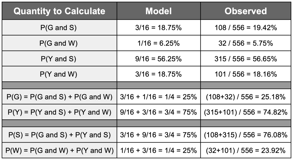
As you can see, all the percentages for the model are close to the ones we obtain from the data collected in Mendel’s experiment. Using these basic quantities, we can also compute the conditional probabilities (having observed one of the traits, how likely we are to get the observed value for the other trait we are considering). This is done for the model, and then compared to the data that we have in the table below.

To give an explicit example, we calculate the probability of the bean being green if we observe it is of a smooth texture. Using Bayes’ Theorem:

P(G | S) =  P(G and S) / P(S) = (108 / 556) / [(108 / 556) + (315 / 556)] = (108/556) / (423/556) = 108 / 423 = 0.2553 or 25.53%

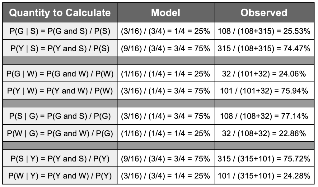
Again, the observed results look fairly close to what we would expect from a Bayes inheritance law with two variables A (type of colour) and B (type of shape), with a ratio of odds of outcomes as in (﹡). These observations made Mendel think that, perhaps, traits are inherited as blocks.

For the same characteristic we can have multiple manifestations (e.g. green and yellow for the colour of the peas); and these different types are what we call alleles. They can be either dominant (in general the outcome for an event with the highest probability, but it is not always the case as we can see for sickle cell anaemia) or recessive. In the case that an individual is born from two parents, it will carry one copy of the genetic material of the trait from each of the parents. If one of the copies carries the dominant variant and the other the recessive one, the dominant one will be the one that is expressed. If two of the same type of allele are present, then that characteristic will be inherited.

Any organism which inherits genetic material from two parents are called diploid, and have two identical sets of different sized chromosomes. On each of the chromosomes, there is an allele which will contribute to the expression of the gene value. So, we inherit two alleles, one from the mother and one from the father, and together they will determine the gene expression.

The scheme of the alleles present on the chromosomes is called the genotype, while the characteristic observed with the naked eye (for example blood type) is called the phenotype. For the blood groups, there are exactly 3 allelic types one can inherit: two dominant ( L^A and L^B) and one recessive (l).

The dominant genes induce the property that the organism’s red blood cells will present certain antigens on the body of the cell (the antigen A is produced under the influence of gene L^A, and the antigen B for the gene L^B, respectively). The recessive gene l has no correspondent antigen.

The corresponding genetic markup for blood type given what alleles we inherit from each parent can be summarized in a table, like the one below.

So, what does this cross-inheritance table actually mean? When you inherit the recessive gene l from both parents, this means you will have no antigens on your red blood cells – hence the blood group is called 0, for “no antigens” (yellow box in the above table).

When instead you have one of the dominant alleles ( L^A or L^B), the corresponding antigens will make an appearance. Now, if you inherit from the other parent the recessive allele (the gene combination will be heterozygous) or the same dominant allele (the combination will be called homozygous), then you will only have one set of antigens on the cells and the letter by which it is called will give the name of the blood group – group A for antigen A; group B for antigen B (these are the red and blue boxes in the table above).

But what happens when you inherit both L^A and L^B – as we can see in the green cells in our table?

When two different, but both dominant alleles are expressed together, the phenotype that this combination will produce will be different from any of the other pairs. This phenomenon is called codominance and can lead to very interesting results. In the case of blood types, they produce a new blood group which we denote by AB, which differs biologically from any of the previously stated blood groups since you will present both antigens A and B on the red blood cells. 

As well as the antigens, the alleles predetermine the type of antibodies present in the plasma: 

• alpha and beta for group O, 
• only beta for group A, 
• only alpha for group B,
• none for group AB.

This little fact actually plays quite an important role in blood transfusions, because the meeting of an antibody and an antigen that are connectable (alpha – A and beta – B), leads to the formation of bonds between them. Since an antibody has 3 possible “docking” sites (imagine it looking like a letter Y), red cells will get stuck together, forming large masses of cells (also called agglutination) that will block the blood vessels and even lead to death.

So, in short, you should know your blood alleles – it might save your life! 

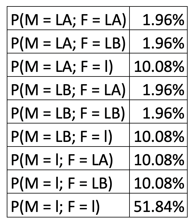
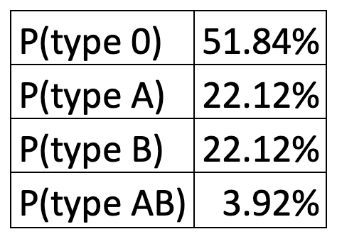
To conclude our discussion, I challenge you to calculate the probabilities of having each of the blood groups, as well as any outstanding conditional probabilities using the following values for the ratios of the alleles L^A : L^B : l  =  7 : 7 : 36  in nature (values taken for Lagos State, Nigeria, between 1998 and 2009, see here). 

(Hint: consider the Allele inherited from the mother and the Allele inherited from the father as two random variables and reuse the logic we employed for calculating those summaries for Mendel’s experiment).

Scroll down for the solution!

.

.

.

.

.

.

.

.

.

.

.

.

Solution

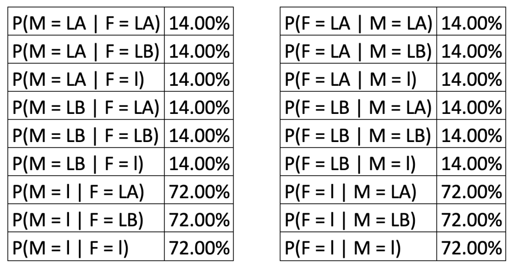
We use F to denote the allele from the father, and M the allele from the mother.