
Lorenzo Piersante
In the previous article we talked about the ways computers can handle basic mathematical operations. This is the result of an ingenious mixture of binary numbers, Boolean logic and electronics.
Thanks to this framework a computer can handle, without breaking a sweat, two groups of operations:
- Arithmetic operations: addition, subtraction, multiplication, division, square root;
- Logical operations: NOT, OR, AND etc.
As we have seen, these operations can be carried out through built-in circuits, so, in a sense, when you program your computer by typing a code, say in Python (making amends to those of you who like old man C++), you tell the machine what circuits do what and in what order, and it doesn’t complain! So, try to be kind to your computer, and don’t ask the impossible, like a division by 0…
Now that we have at our disposal all the basic operations (and a new no-matter-what loyal friend), we might want to consider other operations. Perhaps the two most important operations that undoubtedly we want to perform due to their ubiquitous appearance in the natural sciences and beyond, are: differentiation and integration (you were thinking about these, right!?).
For readers that are not familiar with the meaning and notation of these operations, the pictures below provide a visual summary (or at least they try).
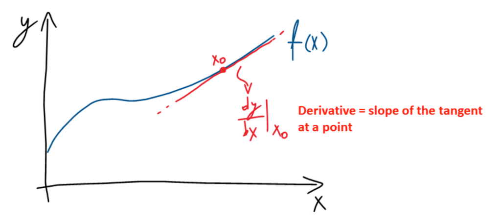

Differentiation and integration are operations on functions, that is curves made up of an infinite number of points. Moreover, the real numbers that compose the function are often made up of an infinite number of digits (e.g. good old π). Therefore, a computer cannot handle them because it does not have infinite memory, nor infinite time available (even if you skip π).
If we want our new best friend to be able to tackle these operations, we must give it some help. We do this by approximating the derivative and integral through some finite-accuracy numerical analogues in the form of approximate algebraic expressions that the computer can manage. The graphs below show what the numerical approximations of the derivative and the integral are:
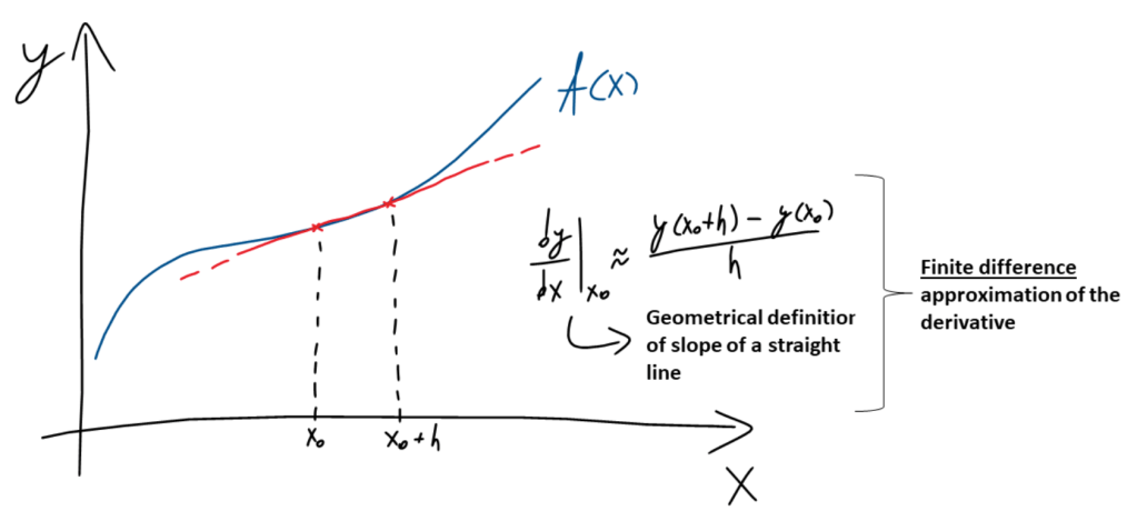
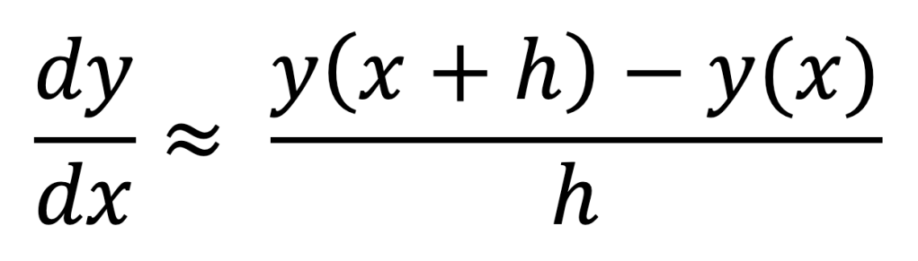
The derivative is approximated by the slope of a straight line passing through the points in the neighbourhood of the point of interest (a secant). In the context of derivatives, numerical schemes of this sort are called finite difference approximations.
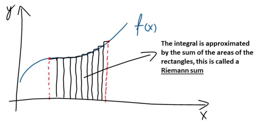
The integral is approximated by the sum of the areas of the rectangles below the curve within the interval of interest, a so-called Riemann sum.
[At this point, the interested reader may want to have a look at the definitions of the derivative and the integral in order to make more sense of the diagrams above.]
The approaches illustrated above go by the name of discretisation: we do not take into account all the points that make up the curve, but only some of them, usually separated by some small fixed distance (h in the approximation of the derivative). Only these points enter the calculations.
Furthermore, the computer will represent these points with some finite accuracy, that is a limited number of digits (in jargon the number is truncated).
Now, using these few ideas we will solve an ordinary differential equation (ODE) by discretising it! The same way a computer program would go about solving it. We will not obtain an analytical solution (i.e. a mathematical expression), but a numerical solution (i.e. a list of numbers) which corresponds to the function that satisfies the equation at the location of the points where the discretisation is carried out.
Let’s consider the following first order ODE:

Subject to the boundary condition y(0) = 1. (y is the function we are trying to solve for).
Don’t worry, my dear interested reader, if you haven’t come across ODEs before, the numerical solution only requires basic algebraic abilities (which is pretty amazing!).
First of all, let’s remind ourselves of the finite difference approximation of the derivative (taken from the picture above):
We set h = 1, and consider the points x = 0, 1, 2, 3, 4, 5 for the discretisation (a regular grid of size 1).
Since h = 1, I need not write the denominator anymore. Then, if we write down the equation for each pair of points by using the finite difference approximation, we obtain the following linear system of equations (the kind of systems of linear equations you have hopefully seen before in high school):

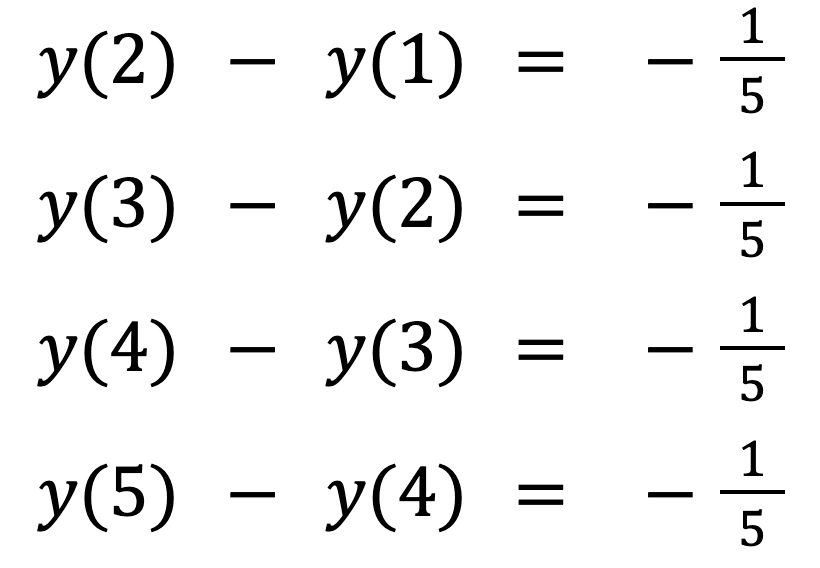
From the first equation we have: y(1) = 4/5.
By substituting this result into the next equation we find: y(2) = 3/5.
Repeating the process for all equations we obtain: y(3) = 2/5, y(4) = 1/5, and y(5) = 0.
The actual solution to the equation is: y(x) = -1/5x + 1.
Sketching a graph of the analytical and numerical solutions, we can see that the agreement is perfect!

We’ve managed to find the value of the solution at the points where the discretisation was carried out without knowing a thing about ODEs, and, more importantly, applying solely operations that a computer is capable of performing!
Pretty amazing, isn’t it? However, a final remark is due. The method above is one of the simplest finite difference schemes that are out there, and it doesn’t always work when the functions become more complex. In these cases, we must apply more sophisticated methods of discretisation in order to be able to solve the equation.
The mathematical notions that we have discussed in this article belong to a branch of Mathematics called numerical methods. Its mission is to study the properties of different discretisation schemes, and to research general purpose approximation procedures for finding numerical solutions to equations. It is a long and fascinating story, and in the next article (COMING SOON), we will begin to scratch the surface of this important area of study…

[…] toolkit of any computer: binary arithmetic and Boolean algebra. Building on this foundation, in the next article of this series, we will demonstrate how a computer can deal with complicated tasks working only with these simple […]
LikeLike
[…] speaking, physical model simulation involves the numerical solution (see the second article of the series for further information) of a complicated differential equation (or a set of them) that describes a physical process […]
LikeLike
Dear
获取 Outlook for iOShttps://aka.ms/o0ukef
LikeLike