
Lorenzo Piersante
As you no doubt are surely aware, computers today are programmed to do all sorts of things. On the pleasant side, we have: video games, video streaming, the web etc. On the serious side (the one we will now explore a little bit further), we have artificial intelligence (AI), computer aided design (CAD), physical model simulation etc.
As the title of this article suggests, the final stage of our journey exploring how computers do maths will be a brief exposure to the numerical procedures that underpin physical model simulation. So, let’s begin!
In the last couple of decades, the availability of more and more powerful computers (titanic machines that can fill an entire building) has allowed the rapid development of the vast area of physical model simulation. That is the branch of the natural sciences and engineering that uses the computational power provided by computers to study physical systems through the solution of their governing equations under various conditions.
Generally speaking, physical model simulation involves the numerical solution (see the second article of the series for further information) of a complicated differential equation (or a set of them) that describes a physical process happening in a region of space.
Numerical methods and computers are essential to this endeavour because, more often than not, it is impossible to find a solution to the equation through conventional analytical methods (i.e. it is impossible to find a mathematical expression that satisfies the equation).
Two common issues encountered are: the geometrical complexity of the object of study or of the region of space, and the conditions the system is subjected to. Numerical procedures are very hand in these circumstances because they can be adapted to complex geometries and conditions with relative ease. Here’s an example…
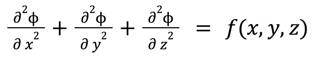
Suppose we want to solve a complicated-looking differential equation, like:
Inside some funny geometrical patch of space like:

Subject to even funnier conditions at each face of this object. Such a problem can, in the general case, be accomplished only through a numerical solution.
To start off the numerical procedure, we must perform some kind of discretisation (see the second article of the series). In this particular instance, we are going to discretise space itself.
From a mathematical point of view, space is continuous, it is made up of an infinite number of points. A computer cannot take them all into account, so we consider only some of them. At these locations we will evaluate through a numerical approximation (refer to the second article of the series for an example of how this is done) the value of the solution to the equation. The picture below shows what this means graphically.
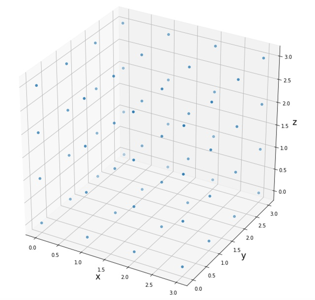
The blue dots indicate the points that will enter the solution algorithm. At these locations we find the value of the solution thanks to the numerical approximation of the derivative.
In order to calculate these numbers, the computer will have to solve a gigantic system of linear equations, similar to the one we met in the second article of the series, with the important difference that the number of equations and variables is many orders of magnitude larger.
If the problem is dynamic, that is if the solution changes with time, a similar discretisation is carried out for time as well. The flow of time is broken down into a finite number of steps, and a solution is found for each of them.
Now that you, my dear interested reader, have been introduced to the concept of space and time discretisation for the purpose of seeking a numerical solution to a differential equation, your efforts for having come so far in this mathematical journey will finally be compensated. And what’s a better compensation than some real-life applications?
Finite difference approximations are a solution method based exactly on what we have talked about in the series so far. A nice example of a simulation based this procedure can be found in this video:
Thanks to our knowledge of Physics and the power of Mathematics, a computer is capable of calculating the seven-year long travel of the ESA space probe BepiColombo to Mercury.
The description of many physical systems involves the conservation of some quantity. In the case of fluid flow, the fluid in question is conserved. Therefore, variations of the method above have been developed to tackle this problem specifically.
Space is discretized in a slightly different manner: not as a collection of points, but as a collection of little volumes that occupy the region of interest (in jargon control volumes or cells). In order to solve the task at hand, a set of linear equations is constructed starting from the amount of stuff that enters and leaves each cell.
The graphic visualisation below demonstrates how the cartesian plane is divided up into a collection of square cells.
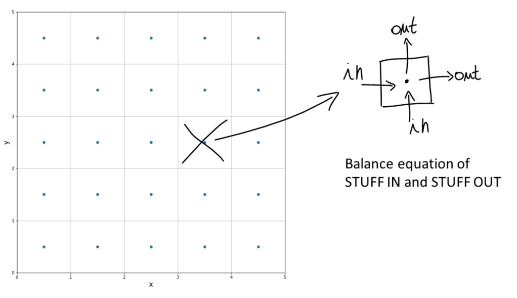
The computer solves the discretised equations and calculates the value of the solution at the centre of each cell. This approach goes by the name of the Finite Volume Method (FVM). As mentioned before, fluid dynamics provides many examples of the application of FVM.
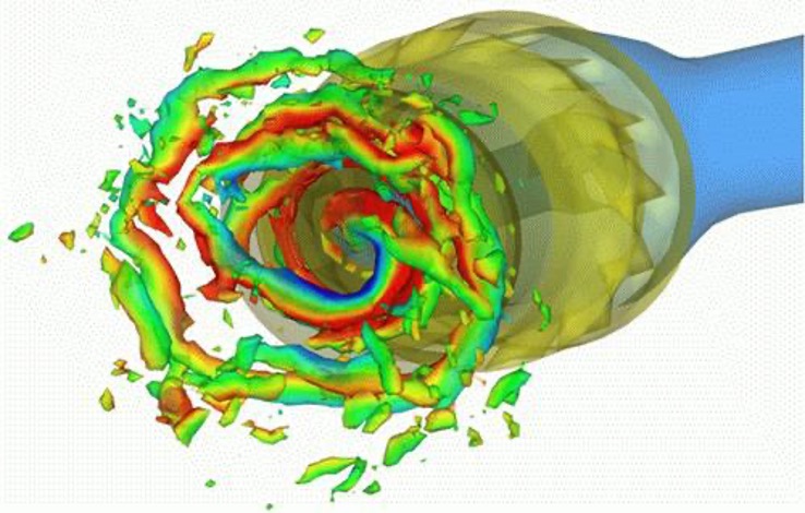
The video below shows an example of a transient simulation of combustion in a furnace.
A final numerical method worth mentioning is Finite Element Analysis (FEA). It is similar to the FVM in the approach to the discretisation of space: the system geometry is broken down into many small cells. However, it differs sensibly from the approaches we have discussed so far, since the computer does not solve the governing equation directly, yet applies a default solution to each cell (which itself satisfies the original equation). The resulting solution is in a sense built block by block (or cell by cell, if you prefer).
From a FEA perspective a rod attached to a wall on one side, and supporting a load on the other, is viewed as follows:
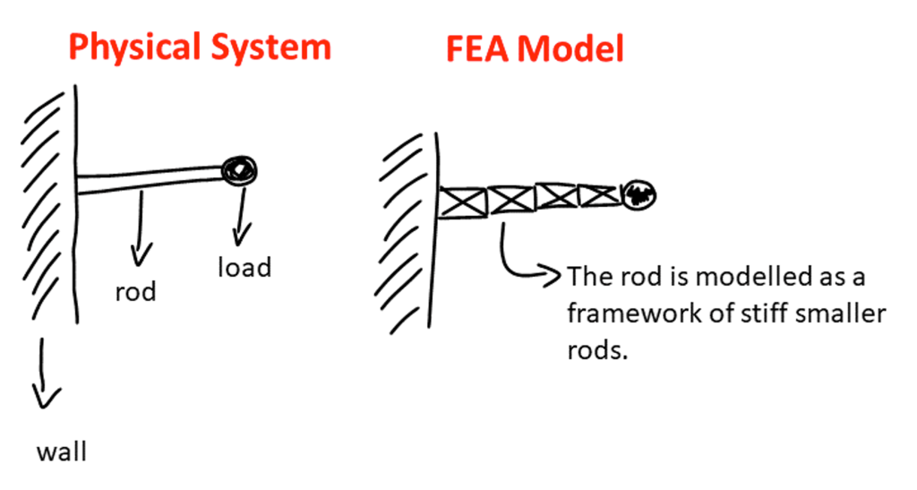
To put it simply, FEA attempts to simplify the system to its fundamental elements.
Despite the perhaps silly-looking appearance of this procedure, it is probably the favourite tool of structural engineers – that is the people who make sure the bridges you walk on don’t collapse under their own weight. Impressive, isn’t it?
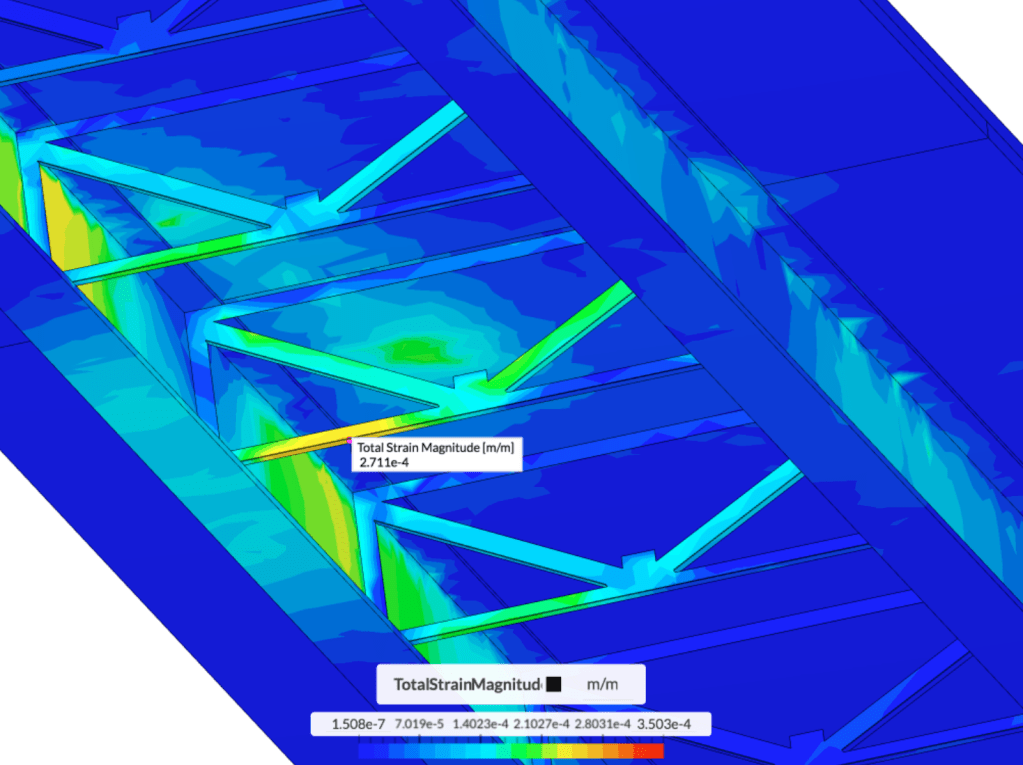
To conclude on the engineristic note, the image below shows a FEA simulation of a bridge traversed by a car. The bright colours in the diagram denote the areas where stronger forces are applied by the presence of the load and the bridge’s structure. You can play with the simulation for yourself here.
With this, my dear interested reader, we conclude our mathematical journey to answer the question: how do computers do maths?
We started by developing a basic understanding of the inner workings of the computing machine, we then delved into the subject of numerical methods, and finally we explored some of most recent applications of computer simulations. And through it all, looking out for us on our journey, was our forever loyal friend: the computer.

Dear
获取 Outlook for iOShttps://aka.ms/o0ukef
LikeLike